 |
 |
 |
 |
 |
 |
The source code count.cc is part of the QCE quantum computing emulator.
Grover's quantum search algorithm [1]
can be used to find solutions to the Boolean function f(x)=1,
where x∈{0,...,N-1} and N=2n
is the number of states represented by n qubits.
But the number of iterations to use in the algorithm depends on the number
of solutions and must be known in advance. Quantum counting [2,3]
is an extension of Grover's algorithm which can determine the number of solutions.
Variations of quantum counting can also be used to find the mean of a function
[4], evaluate multidimensional integrals [5],
and perform quantum Monte Carlo simulations [6].
Let G represent the Grover operation of phase flip and inversion about
the mean. To count the number of solutions t
to f(x)=1, first initialize two
registers to the state (H|0m>)H|0n>
using n qubits for the input x of function f(x),
and m qubits for an auxiliary counter.
Construct the state |j>(Gj|x>),
then apply the inverse quantum Fourier transform (QFT) to the |j> register,
then measure that register and denote the outcome y [3].
The estimated total amplitude of the solution states is a=sin(πy/M)
and the estimated number of solutions is t=Na2,
where N=2n and M=2m.
The accuracy of the estimate depends on the number of qubits m used
for the auxiliary register.
The QFT result will be symmetric about the state index M/2,
thus there will be pairs of measurement results for y which will produce
the same estimate t. In general the estimated t value
will not be an integer and must be rounded to the nearest integer. Letting
P represent the total probability that the measured and rounded estimated
t values equal the true value, simulation results demonstrate increasing accuracy as
the size of the auxiliary register increases:
 |
 |
 |
 |
 |
 |
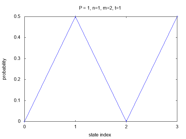
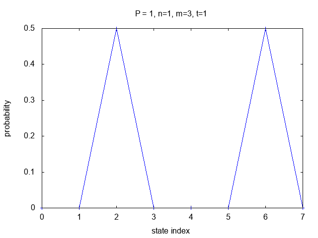
In the top-left first two cases shown above, t/N=1/2
which results in the estimated t value being an integer
and the total probability of a correct measurement is 1.
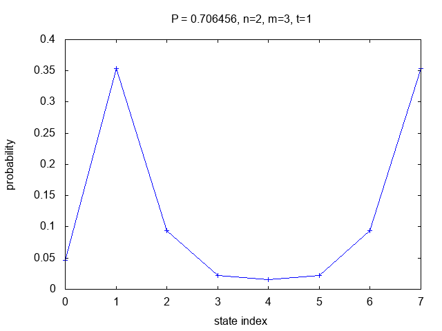
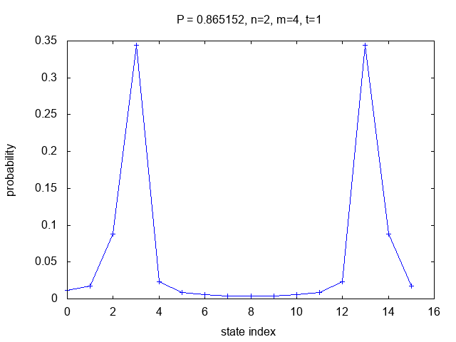
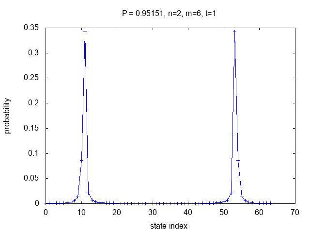
The other cases use t/N=1/4 with increasing
values of m and increasing accuracy of the results.
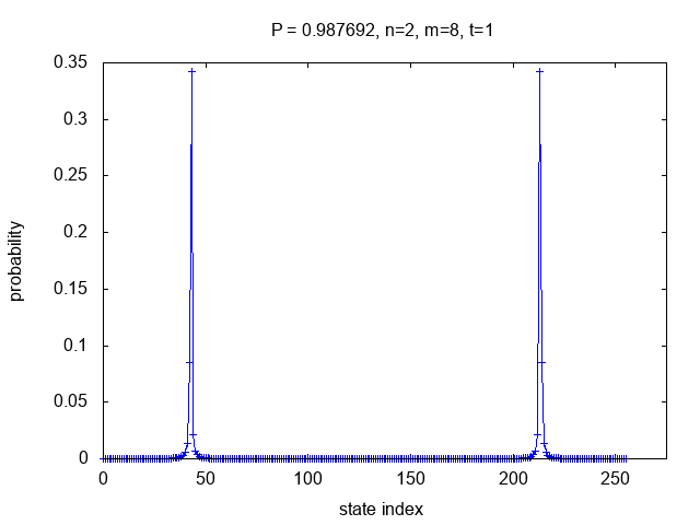
Besides the two primary peaks in the probability plots, other
points near the peaks also result in estimated t values
which when rounded are correct. For example, in the bottom-right case
for m=8,
the peaks at state indices 43 and 213 each contribute 0.341968 to the total probability,
but there are 46 additional points near those peaks which also round to the correct
estimate and the total probability is 0.987692.
The raw simulation output shows the input parameters followed by
the state indices and probabilities to be plotted, followed by lines marked "count:"
with the state data sorted by increasing probability, including estimated and
rounded t values, and ending with the total probability (pt and 1-pt), theoretical
peak state index values (ek), and the mean and standard deviation of the unrounded
estimated t values.
To compare quantum counting with classical Monte Carlo, consider a simulation of
blackjack using two cards drawn from an infinite deck. There are 13 possibilities
for each card {A,2,...10,J,Q,K} and 8 ways to get blackjack: A and 10,J,Q,K; or 10,J,Q,K and A.
8 qubits are required for the Boolean function implementation, 4 for each card,
plus m additional qubits for the QFT register, where
M=2m is the equivalent sample size for a classical simulation.
The exact solution count is t=8, corresponding to the probability
p=8/(13*13). A classical Monte Carlo simulation using M
trials with S successes will estimate the probability as S/M
which corresponds to an estimate 13*13*S/M for the solution count.
As in the quantum case, the classical estimated t value must be rounded
to the nearest integer. The total probability of a correct classical estimate is:
P(7.5 ≤ 13*13*S/M ≤ 8.5) = P(⌈7.5*M/169⌉ ≤ S ≤⌊8.5*M/169⌋)which is computed as a sum of binomial probabilities by bj.m.
The standard deviation of unrounded estimates can be computed from the QFT result
probabilities in the quantum case, and in the classical case is:
169*sqrt(p*(1-p)/M).
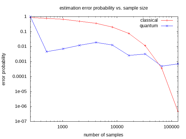
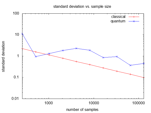
Evaluating the estimation error probability (1-P) and standard deviation
for M=256,512,...,131072 (m=8,9,...,17 qubits)
shows that the classical case has higher error below
M=65536 (m=16 qubits)
but generally lower standard deviation:
 |
 |
Theoretically the quantum approach should have estimation error O(M-1)
which is a quadratic improvement over the classical error O(M-1/2),
as seen for example in [6] Figure 11. But that theoretical
improvement is based on assumptions and bounds which do not apply here.
Theoretically the log-log classical estimation error curve should be linear,
but here it was computed using the exact binomial formula including rounding effects
and it exhibits enhanced performance for increasing sample size.
On the other hand, the quantum estimation error and standard devisation do not improve
as much as expected for increasing sample size, which is hard to explain
and may be due to an implementation bug.
The quantum simulation run-time increases by about a factor of 4 for each additional qubit up to 4260 seconds (1 hour, 11 minutes) for 17 qubits:
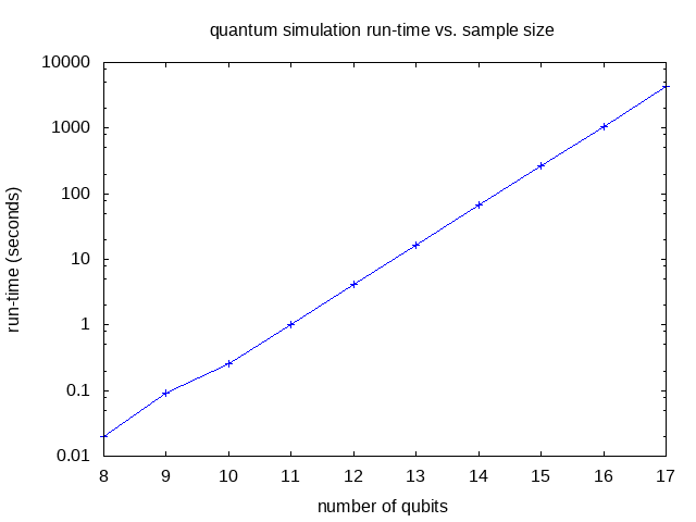
Quantum Simulation Run-time
The run-time of a physical quantum computer for this application is O(M)
due to the M Grover Gj operations,
which increases the run-time by a factor of 2 for each additional qubit.
But a quantum simulation requires O(M2) operations overall,
since each simulated Grover step itself takes O(M) operations.
A multi-core/multi-node implementation would be needed for simulations using larger numbers
of qubits to run in a reasonable amount of time.
[1] Grover's algorithm, Wikipedia, https://en.wikipedia.org/wiki/Grover's_algorithm
[2] Quantum Counting, Gilles Brassard, Peter Hoyer, and Alain Tapp, May 1998, https://arxiv.org/abs/quant-ph/9805082
[3] Quantum Amplitude Amplification and Estimation, Gilles Brassard, Peter Hoyer, Michele Mosca, and Alain Tapp, May 2000, https://arxiv.org/abs/quant-ph/0005055
[4] An optimal quantum algorithm to approximate the mean and its application for approximating the median of a set of points over an arbitrary distance, Gilles Brassard, Frederic Dupuis, Sebastien Gambs, Alain Tapp, June 2011, https://arxiv.org/abs/1106.4267
[5] Fast quantum algorithms for numerical integrals and stochastic processes, Daniel S. Abrams, Colin P. Williams, Aug. 1999, https://arxiv.org/abs/quant-ph/9908083
[6] Option Pricing using Quantum Computers, Nikitas Stamatopoulos, Daniel J. Egger, Yue Sun, Christa Zoufal, Raban Iten, Ning Shen, and Stefan Woerner, July 2020, https://arxiv.org/abs/1905.02666