Time-varying Gauss-Markov Channel Coefficients
Last Modified:
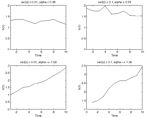
 The top two plots show examples of how h(1) can vary over time
depending on the variance of the Gaussian part of the
Gauss-Markov distribution. The mean of h(1) is constant.
In the bottom two plots,
after initializing h at time 1 using alpha = 0.95,
alpha was changed to 1.08 to generate the coefficients.
This causes the mean of h(1) to increase over time.
Time-varying Gaussian Channel Coefficients
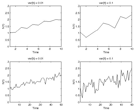
 In the above four plots, h(1) is Gaussian with mean varying
linearly from 1 to 2 over the block of time. The bottom two
plots show examples over a longer time scale.
