Following are the results of some Monte-Carlo simulations related to the report "EM ISI Examples, R. Perry, 18 April 1999".
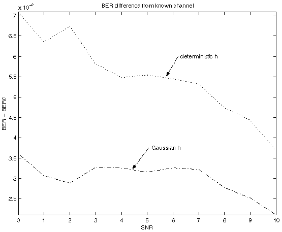
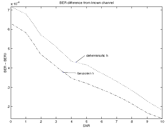
Using 100000 trials, with two iterations of each algorithm for each trial, and L=3, with h generated as independent Gaussian random variables with mean 1 and variance 0.5, and (-1,1) data values generated with p(1)=p(-1)=0.5 for each trial, with N=6, BER results are:
                       EM algorithm
  SNR      deterministic h      Gaussian h        known channel
   0       0.2445               0.24527           0.23782
   1       0.22147              0.2217            0.21476
   2       0.19905              0.1986            0.19306
   3       0.17598              0.175             0.17051
   4       0.15159              0.15029           0.14622
   5       0.12737              0.12615           0.12228
   6       0.10418              0.10252           0.098812
   7       0.082693             0.08176           0.078048
   8       0.064388             0.063047          0.05977
   9       0.049082             0.047553          0.045163
  10       0.037187             0.035667          0.033837
Here is a plot corresponding to the above table, showing BER-BER0
where BER0 is the known channel result:
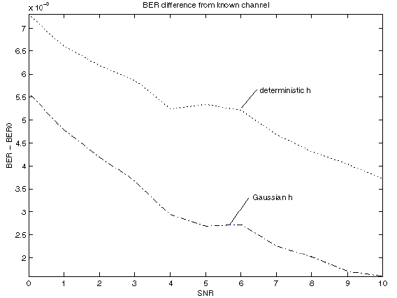
Results with h generated as correlated Gaussian random variables with autocorrelation matrix:
  Rh =
          0.5         -0.5            0
         -0.5            1         -0.5
            0         -0.5            1

                       EM algorithm
  SNR      deterministic h      Gaussian h        known channel
   0       0.23844              0.23664           0.23164
   1       0.21629              0.2149            0.20943
   2       0.19276              0.19217           0.18673
   3       0.16909              0.16806           0.1632
   4       0.14546              0.14467           0.13981
   5       0.12275              0.12252           0.11727
   6       0.1001               0.099793          0.095015
   7       0.080307             0.079165          0.075267
   8       0.062903             0.061647          0.057837
   9       0.048963             0.047653          0.044485
  10       0.038915             0.037535          0.03511
and the corresponding plot:
We also measured the number of occurrences of bit errors vs. bit position in the time sequence of received data. These errors were consistently significantly higher for the initial bits, then significantly lower for the final bits, using the Gaussian EM algorithm as compared to the deterministic algorithm. No explanation for this pattern of bit errors has yet been found.
| (22)  f(h|r,B) = K4 exp(-(h-g)'(B'B/s+inv(Rh))(h-g)/2)
|
| where K4 is a constant scale factor,
| and we are assuming that E[h|r,B] = E[h].
The assumption that
g=E[h] was made in order to simplify the result.
But that assumption is not necessary, and is wrong if E[h] is known apriori.
It corresponds to the case where E[h] is unknown, so E[h|r,B] must be
estimated solely from the received data and estimate of B using pinv(B) r.
This may have some usefulness, but it seems difficult to justify a case where f(h) is known to be Gaussian, with known autocorrelation matrix and unknown mean. Nevertheless, the simulation results for this case show that the EM algorithm works better than the algorithm for deterministic h, so we are including the following results for possible future use.
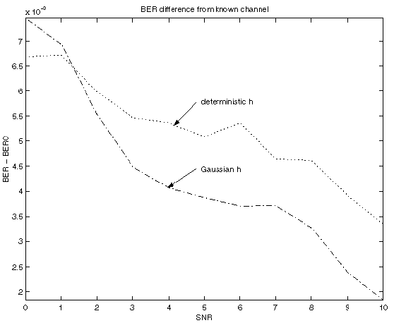
Using 100000 trials, with two iterations of each algorithm for each trial, and L=3, with h generated as independent Gaussian random variables with mean 1 and variance 0.5, and (-1,1) data values generated with p(1)=p(-1)=0.5 for each trial, with N=6, BER results are:
                       EM algorithm
  SNR      deterministic h      Gaussian h        known channel
   0       0.24334              0.24163           0.23604
   1       0.22204              0.22022           0.21544
   2       0.20003              0.19804           0.19384
   3       0.17561              0.17341           0.16974
   4       0.1518               0.1495            0.14656
   5       0.12812              0.12547           0.12278
   6       0.10481              0.10232           0.099597
   7       0.08226              0.079847          0.077582
   8       0.063602             0.061307          0.059287
   9       0.048818             0.046478          0.044768
  10       0.037373             0.035263          0.033662
Here is a plot corresponding to the above table, showing BER-BER0
where BER0 is the known channel result:
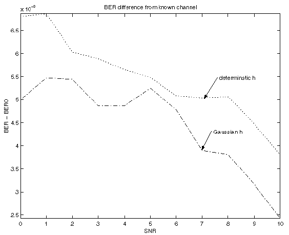
Results using N=10 with all other parameters the same as above are:
                       EM algorithm
  SNR      deterministic h      Gaussian h        known channel
   0       0.23123              0.23036           0.22406
   1       0.20988              0.20891           0.20308
   2       0.18584              0.18483           0.18014
   3       0.16023              0.1592            0.15513
   4       0.13527              0.13439           0.13093
   5       0.10961              0.10865           0.10545
   6       0.085422             0.084591          0.081701
   7       0.065108             0.064349          0.061806
   8       0.0475               0.046814          0.044667
   9       0.034066             0.033447          0.031785
  10       0.023925             0.023479          0.022104
Plot for N=10:
  Rh =
          0.5         -0.5            0
         -0.5            1         -0.5
            0         -0.5            1


                       EM algorithm
  SNR      deterministic h      Gaussian h        known channel
   0       0.23887              0.23539           0.23178
   1       0.21588              0.21259           0.20953
   2       0.19307              0.1892            0.18632
   3       0.16919              0.16665           0.16338
   4       0.14464              0.14241           0.13916
   5       0.1218               0.11941           0.11626
   6       0.099057             0.096868          0.093613
   7       0.080172             0.078062          0.074848
   8       0.063065             0.06111           0.058335
   9       0.04975              0.04783           0.045313
  10       0.038383             0.036812          0.034715
and the corresponding plot: