CORVIDS (COmplete Recovery of Values In Diophantine Systems) is a method for recreating data from statistics such as mean and standard deviation [1,2]. It performs an exhaustive search over the space of possible solutions which can be computationally expensive. Here we describe the CORVIDS method and show examples using Grover's quantum algorithm to perform the search.
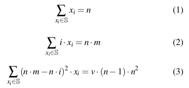
CORVIDS finds all non-negative integer solutions x to the equations [2]:

where xi is a count of number of occurrences of response i, for i=1...r, n is the total number of responses, m is the reported mean, and v is the reported variance. In matrix form the equations are Ax=b. For example, with n=20, m=1.85, v=0.8750942 and responses on a 1 to 7 scale (r=7):
| Ax = |
|
|
= |
|
= b |
Solutions are found by performing a unimodular transformation P on an augmented matrix G to reduce it to Hermite form H [3]:
| P G = |
|
|
= |
|
= H |
| P = |
|
H = |
|
| y = |
|
RT = |
|
All solutions may then be written as x = y + RTc and we would like to find all
possible values of c which produce non-negative values for x.
CORVIDS does this by transforming R to reduced row echelon form,
creating a new y solution with rank(R) zeros,
and then using a search with pruning over the space of possible c values [2]:
| y = |
|
RT = |
|
The search for solutions need only consider values of c such that 0 ≤ ci ≤ n and ∑ ci ≤ n. Furthermore, when incrementing ci to generate potential c values, if ci=v and any xj is negative and the corresponding Rij value is also negative, the range v+1 ≤ ci ≤ n may be skipped since those values would just make xj more negative.
In this example, out of 10312 potential values of c considered, we obtain 4 solutions, xT =
  [6, 13, 0, 0, 1, 0, 0]
  [7, 11, 0, 2, 0, 0, 0]
  [8,  8, 3, 1, 0, 0, 0]
  [9,  5, 6, 0, 0, 0, 0]
To handle reported statistics which have been rounded, CORVIDS allows tolerances to be specified for the mean and/or variance, and it solves separate sets of equations for each valid mean/variance pair [2].
A quantum computer could use the Grover search algorithm to solve equations (1-3) directly,
with quantum registers xi initialized to a superposition of possible
values 0...n, a quantum oracle to flip the phase of values which satisfy the equations,
and an inversion about the mean operation.
Approximately
(π/4)sqrt(N/M) iterations would be required
(for large N and small M),
where N=2p and M is the number of solutions [6, page 254].
The number of qubits required to represent x is
p=⌈log2(n+1)⌉r.
For the numerical example above, with n=20 and r=7, we have p=35,
and with M=4 approximately (π/4)sqrt(235/4)=72792
iterations would be required. This performance is worse than the classical CORVIDS
algorithm which searched only 10312 potential values of c, however it
skips the reductions to Hermite and row echelon forms.
If we first use classical CORVIDS to reduce the problem to
x = y + RTc, with
R in reduced row echelon form,
then the quantum search for the rank(R) values of c
would require
p=⌈log2(n+1)⌉rank(R) qubits,
that is p=20 and only (π/4)sqrt(220/4)=402 iterations
for the example above.
This is better, but in any case note that measurement of the quantum result will yield only one of the possible solutions, even if the final state is a superposition of multiple solutions. The search would have to be repeated multiple times to obtain a random sampling of solutions.
The optimum number of iterations depends on the number of solutions, which is not known in advance. And performing too many iterations decreases the probability of measuring a correct result. However, using a quantum counting algorithm similar to the Grover search [6, section 6.3], it is possible to first determine the number of solutions, and then perform the search.
Note that the classical CORVIDS implementation displays only a small random selection of the results if there are more than 20 solutions. In a case where there are an excessive number of solutions one might prefer a statistical summary of the results. In the quantum case we will only obtain one result upon measurement, so maybe that result should be an average instead of a specific answer?
In the simulations below we assume that the sums of valid solution coefficients can be tracked by a quantum algorithm, and we show the sums, associated probability of measurement, and average coefficient values (sums divided by the number of solutions).
In the following examples the dimension is rank(R),
i.e. the dimension of the nullspace N(A), which is the number
of c values to be determined.
Starting with response counts xT=[5, 1, 1], we have n=7 and mean m=(5*1+1*2+1*3)/7=1.4286. Using classical CORVIDS with no variance specified, two solutions are found, xT =
  [4, 3, 0]
  [5, 1, 1]
| x = y + RTc1 = |
|
+ |
|
|
Using input data corvids-c1.in, with 3 qubits to represent the possible c1 values 0...7, the simulated quantum computer output shows the state values, probabilities (magnitude squared of amplitude), and complex amplitudes for two iterations of the Grover algorithm. After one iteration the only states with non-zero probability are the solutions c1=4 and c1=5:
  inv (sorted):
     0   0 (0,0)
     1   0 (0,0)
     2   0 (0,0)
     3   0 (0,0)
     6   0 (0,0)
     7   0 (0,0)
     4   0.5 (0.707107,0)
     5   0.5 (0.707107,0)
  sum:
     9   1
  avg:
   4.5
Starting with response counts xT=[1, 2, 3, 1], we have n=7 and mean m=(1*1+2*2+3*3+1*4)/7=2.5714. Using classical CORVIDS with no variance specified, ten solutions are found, xT =
  [0, 3, 4, 0]
  [0, 4, 2, 1]
  [0, 5, 0, 2]
  [1, 1, 5, 0]
  [1, 2, 3, 1]
  [1, 3, 1, 2]
  [2, 0, 4, 1]
  [2, 1, 2, 2]
  [2, 2, 0, 3]
  [3, 0, 1, 3]
  [0, 3]
  [0, 4]
  [0, 5]
  [1, 1]
  [1, 2]
  [1, 3]
  [2, 0]
  [2, 1]
  [2, 2]
  [3, 0]
| x = y + RTc = |
|
+ |
|
|
  inv (sorted):
  ...
     5   7   0.00219727 (0.046875,0)
     6   7   0.00219727 (0.046875,0)
     7   7   0.00219727 (0.046875,0)
     0   3   0.0881348 (0.296875,0)
     0   4   0.0881348 (0.296875,0)
     0   5   0.0881348 (0.296875,0)
     1   1   0.0881348 (0.296875,0)
     1   2   0.0881348 (0.296875,0)
     1   3   0.0881348 (0.296875,0)
     2   0   0.0881348 (0.296875,0)
     2   1   0.0881348 (0.296875,0)
     2   2   0.0881348 (0.296875,0)
     3   0   0.0881348 (0.296875,0)
  sum:
    12  21   0.881348
  avg:
   1.2 2.1
This example uses the reduced data from the classical CORVIDS example at the beginning of these notes. Each of the four c coefficients requires 5 qubits to represent the possible values 0...20, that is 4*5=20 qubits total.
Using input data corvids-c4.in, the simulated quantum computer output shows the main results after 402 iterations of the Grover algorithm.
  final (sorted):
  ...
    29  31  31  31   2.06164e-12 (-1.43584e-06,0)
    30  31  31  31   2.06164e-12 (-1.43584e-06,0)
    31  31  31  31   2.06164e-12 (-1.43584e-06,0)
     6  13   0   0   0.249999 (0.499999,0)
     7  11   0   2   0.249999 (0.499999,0)
     8   8   3   1   0.249999 (0.499999,0)
     9   5   6   0   0.249999 (0.499999,0)
  sum:
    30  37   9   3   0.999998
  avg:
   7.5 9.25 2.25 0.75
The carrots case study from SPRITE [5]
has n=45, mean m=19.4, and variance v=19.92.
Using response values 0, 1, 2, ..., 55 (number of carrots taken) and no tolerance
specified on the mean and variance, there are no exact solutions.
Allowing a tolerance ±10 on the variance, CORVIDS finds solutions,
but rank(R)=53 and the search space
is of size 4653 ~= 2293 so an exhaustive search is infeasible.
A quantum search would require 6*53=318 qubits which is infeasible to simulate but
could be performed easily on a physical quantum computer of sufficient size.
If we represent the carrots in multiples of 5, i.e. using response values 0, 5, 10, ..., 55,
and round the mean and variance to 20 and 202 respectively,
CORVIDS finds solutions with rank(R)=9 so the search space
is of size 469 ~= 250 which is barely feasible.
A quantum search would require 6*9=54 qubits which is infeasible to simulate but
could be performed easily on a small physical quantum computer.
[1]
Computer algorithms
can test the dodginess of published results, The Economist, June 2018:
As they describe in a paper in PsyArXiv Preprints,
Sean Wilner and his colleagues at the University of Illinois at Urbana-Champaign have come
up with a way of reconstructing, given the mean, standard deviation and number of data points
in a result (all three of which are usually stated as part of such a result), all the
possible data sets which could have given rise to that result.
The PsyArXiv paper is [2] Complete recovery of values
in Diophantine systems (CORVIDS), Sean Wilner, Katherine Wood, and Daniel Simons,
July 02, 2018. The software is available at
github.com/katherinemwood/corvids. It uses a version of
[3] Diophantine
by Thomas G. Close for finding small solutions of systems of diophantine equations,
which is based on the LLL algorithm from
[4] Extended gcd
and Hermite normal form algorithms via lattice basis reduction, G. Havas, B.S. Majewski, and
K.R. Matthews, Experimental Mathematics, Vol 7 (1998) 125-136.
A related heuristic method is described in
[5] Recovering data from summary statistics:
Sample Parameter Reconstruction via Iterative TEchniques (SPRITE),
James A Heathers, Jordan Anaya, Tim van der Zee, and Nicholas JL Brown,
PeerJ Preprints, May 30, 2018.
[6] Quantum Computation and Quantum Information, 10th Anniversary Edition, Michael A. Nielsen & Isaac L. Chuang, Cambridge University Press, 2010.