High-level Quantum Computing Emulation for Evaluation of Quantum Algorithms

High-level quantum computing emulation is described and simulation results are presented for some applications, including phase shift and depolarization errors.

In a physical quantum system the 2ⁿ states can not be observed directly. They collapse into a single value when measured, based on the complex amplitude squared, which corresponds to the probability of the measured value. In a simulation however we can manipulate and view the state amplitudes directly, providing insight into the internal operation of quantum algorithms.

Quantum operations can be described mathematically using unitary matrices, but such 2ⁿ-by-2ⁿ matrices are not practical to use directly in a simulation, so alternatives using sparse storage or decision diagram representations may be employed. Here we follow the method described in [1] and use classical function evaluation where appropriate instead of low-level quantum gate simulation, and no matrices are required.

For example, consider the quantum operation of addition mod M: (a,b)->(a,(a+b)%M), where a and b are m-qubit pieces of an n-qubit register q, with n=2m, N=2ⁿ, and M=2^m. A low-level quantum implementation of addition is described in [2] and is rather complicated. But a high-level simulation can be performed simply using classical addition; in C pseudo-code:

  t = copy(q); // temporary copy of q register

  for( X = 0; X < N; ++X) // for each element of the state array
  {
    a = X >> m;       // top m bits
    b = X & mask;     // bottom m bits, mask = 2m-1 = 0111..1 (m 1's)
    c = (a + b) % M;  // classical addition
    Y = (a << m) | c; // concatenate the bits
    q[Y] = t[X];      // perform the permutation
  }

  q    a   b  ->  a (a+b)%2
  0    0   0      0   0
  1    0   1      0   1
  2    1   0      1   1
  3    1   1      1   0

Functions which do not represent a permutation may also be simulated directly at a high-level. The quantum discrete Fourier transform can be simulated by simply performing a classical DFT on the state array coefficients. The phase flip and inversion about the average used in Grover's algorithm can be simulated at a high-level by simply performing the computations; in C pseudo-code:

    q[m] = -q[m]; // apply f, i.e. flip sign of state m

    a = 0; for( i = 0; i < N; ++i) a += q[i];

    a *= 2.0/N; for( i = 0; i < N; ++i) q[i] = a - q[i]; // inversion about the average

Compared with a low-level quantum circuit for the Grover iteration (from [15]), the high-level simulation does not require any Hadamard transformations or other gates, and also does not require use of auxiliary oracle workspace qubits.

The resulting quantum state is the same regardless of whether it is simulated at a low-level or high-level.

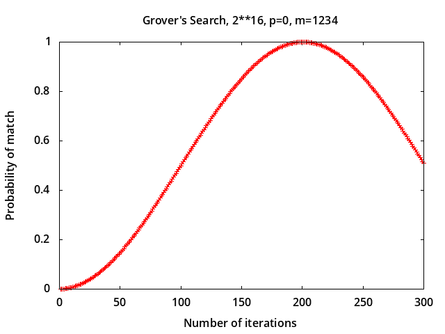
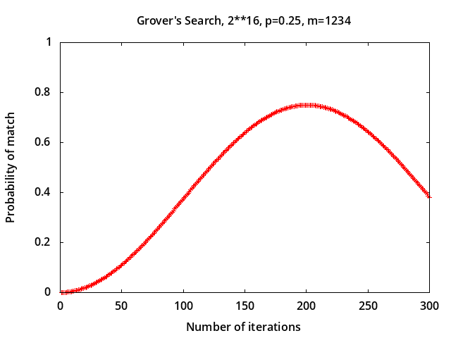
Grover's search - simulation results for searching a 16-bit space, i.e. 2¹⁶ = 65536 possibilities, which would take (2¹⁶)/2 = 32768 iterations on average using a classical algorithm. The quantum algorithm takes only (π/4)2^16/2 = 201 iterations optimally to find a match with a probability of 0.999988 with no noise (top left plot); additional iterations reduce the probability. In the plot on the top right, depolarizing noise level p = 0.25 reduces the probability of match to 0.749995.

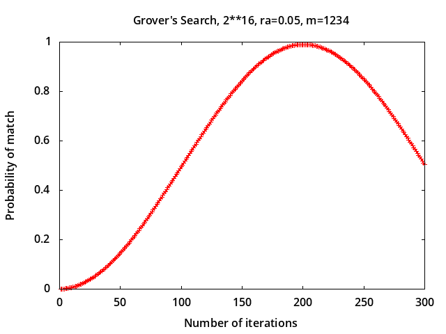
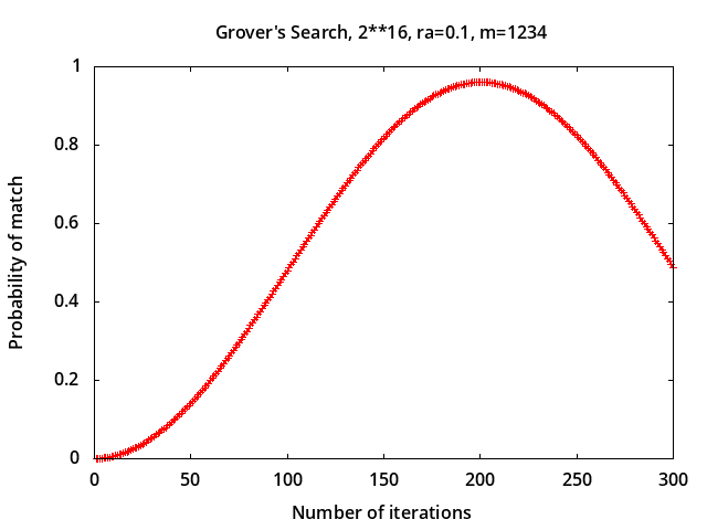
The bottom plots show the effect of errors caused by non-resonant pulses implementing the initial Hadamard transformations (see notes on Magnetic Pulse Error Analysis). For relative error ra=0.05 the probability of match after 201 iterations is 0.990014 and for ra=0.1 it is 0.960394.

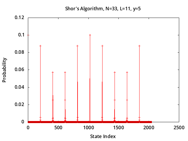
Shor factoring - simulation factoring N=33 using L=11 work qubits and y=5 (order 10). DFT probability peaks occur at (205, 410, 614, 819, ...), and dividing those into 2¹¹ produces period estimates (9.9902, 4.9951, 3.3355, 2.5006, ...). Using r = 10 ≈ 9.9902 we have y^r - 1 = 0 (mod N), so (y^r/2 - 1)*(y^r/2 + 1) = (5⁵ - 1)*(5⁵ + 1) = 22*24; gcd(22,N) = 11, gcd(24,N) = 3, both factors of N.

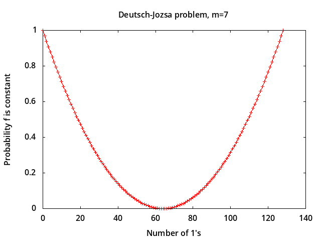
Deutsch-Jozsa problem - simulation results for P(constant) vs. number of 1's in the output of a hidden Boolean function. The hidden function is supposed to be either constant (always 0 or always 1) or balanced (0 for half of the possible inputs and 1 for the other half). For a function with m input bits, a classical solution must call the function up to 1+2^m-1 times to determine if it is constant or balanced. But the quantum solution can do it with just one function call, regardless of the size of m. Results shown are for randomly generated functions with 0 to 2^m 1's in their output, so the two end points represent constant functions and only the middle point represents a balanced function. The plot shows the probability varying smoothly between 1 and 0 for the non-constant/non-balanced functions indicating that this algorithm may usefully detect functions which are almost constant or balanced.

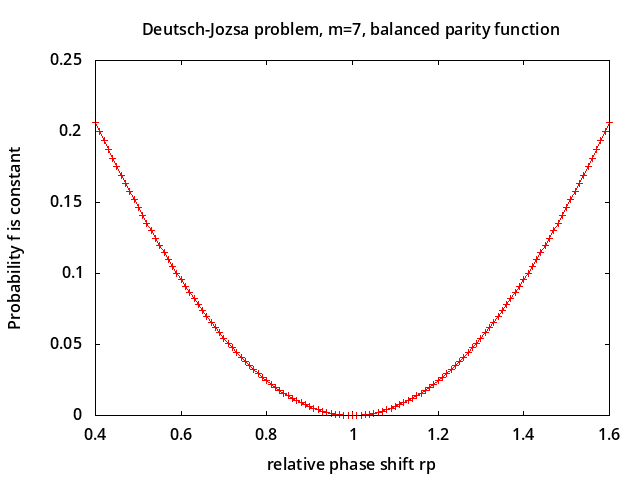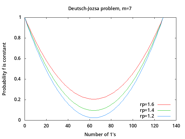
The plots above show P(constant) when there is a phase shift error implementing the Hadamard transformations (see notes on Magnetic Pulse Error Analysis). The relative phase shift is rp=φ/(π/2) so rp=1 represents no phase shift error. For non-constant functions the phase shift error causes P(constant) to increase, so for balanced functions it is greater than 0. In the left plot, for Number of 1's = 64 (i.e. balanced functions), P(constant) is 0.0244717, 0.0954915, 0.206107 for rp = 1.2, 1.4, 1.6 respectively. The plot on the right shows P(constant) for the parity function, which is balanced, for a range of phase shift errors.

Also see notes on Deutsch-Jozsa Coin Analogy.

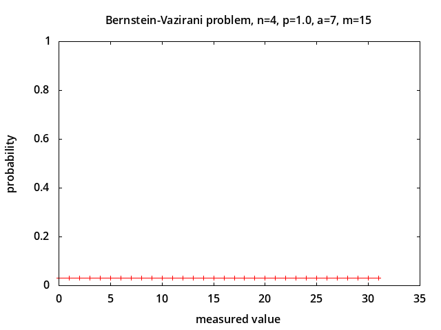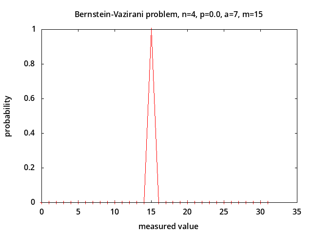
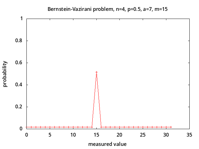
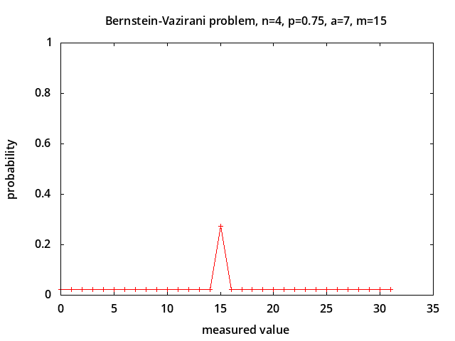
Bernstein-Vazirani problem - determine parameter a in the hidden parity function f(x) = a · x ⊕ b [7] in the presence of depolarizing noise [12]. This problem is considered to be intractable classically. The probabilities of measured values for noise levels p = 0.0, 0.5, 0.75, 1.0 are shown above for a = 7 corresponding to correct measured value m = 2*a + 1 = 15. With no noise (p = 0.0) the correct value is always measured. With 100% noise all possible measured values are equally likely with probability 1/2ⁿ⁺¹ (0.03125 for n=4). The probability of measuring the correct value is linearly related to the noise level: P(m) = (1-p)*1.0 + p/2ⁿ⁺¹.

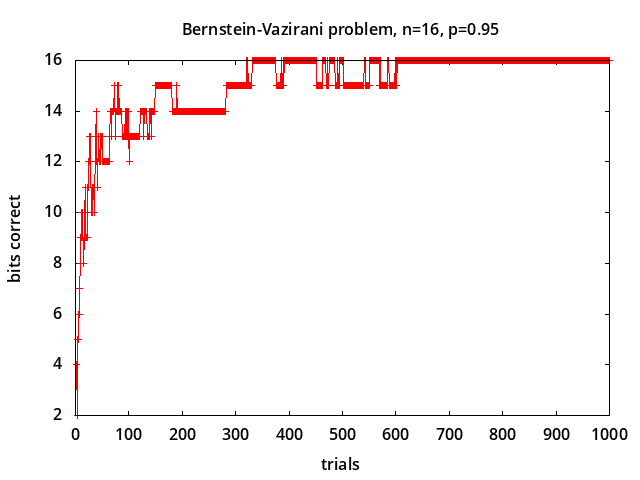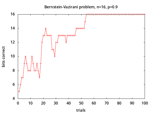
In the simulations shown above, each trial represents a measurement, and the 16-bit parameter is estimated using a bit-wise majority vote following [12]. In the examples shown, for noise level 0.9 all bits are correct after about 60 trials, and for noise level 0.95 all bits are correct after about 650 trials.

The Bernstein-Vazirani algorithm is performed just once, and then repeated measurements are simulated based on the state probabilities (amplitudes squared). Unlike a physical quantum system, simulated measurements do not collapse the state, so multiple measurements may be performed without redoing the algorithm.

Depolarization produces a mixed state which can not be represented using a state vector (see notes on Depolarization and Mixed States). And according to [12], depolarization should be performed before the final Hadamard transformation. But unitary transformations have no effect on a depolarized density matrix, since U*I*U^† = U*U^† = I.

So depolarization is simulated after H, just before measuring, by creating a state which will lead to proper measurements, changing each state amplitude A using a convex combination, so |A| becomes sqrt((1-p)*|A|² + p*h²) and the phase becomes (1-p)*∠A + p*0, where h² = 1/2ⁿ⁺¹.

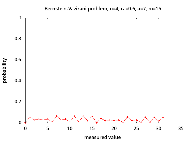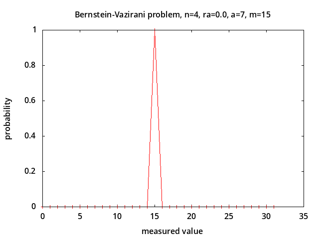
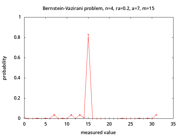
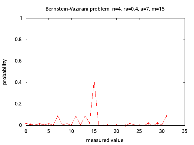
The plots above show the probabilities of measured values with non-resonant pulses implementing the Hadamard transformations for different relative error levels r_a. (see notes on Magnetic Pulse Error Analysis). With no error (r_a = 0.0) the correct value is always measured. For r_a = 0.2, 0.4, 0.6 the probability of measuring the correct value is 0.828412, 0.417071, 0.0647358 respectively.

[1] High Performance Emulation of Quantum Circuits, Thomas Häner, Damian S. Steiger, Mikhail Smelyanskiy, Matthias Troyer, 2016. Uses classical function evaluation instead of low-level quantum gate simulation.

[2] A new quantum ripple-carry addition circuit, Steven A. Cuccaro, Thomas G. Draper, Samuel A. Kutin, David Petrie Moulton, 2004. An example of a low-level implementation. This is reference #12 from [1].

[3] An Introduction to Quantum Algorithms, Emma Strubell, 2011. Has detailed small example of Grover's algorithm.

[4] Python Quantum Computing simulator, Juliana Peña, 2011. Two qubits and superdense coding protocol example. Errata.

[5] An Introduction to Quantum Computing, Without the Physics, Giacomo Nannicini, Nov 2018.

[6] The Deutsch-Jozsa Problem: De-quantisation and Entanglement, Alastair A. Abbott, 2010.

[7] Quantum algorithms revisited, R. Cleve, A. Ekert, C. Macchiavello, M. Mosca, Proc. R. Soc. Lond. A (1998) 454, 339-354. This is reference #6 from [6].

[8] A pseudo-simulation of Shor's quantum factoring algorithm, J.F.Schneiderman, M.E.Stanley, P.K.Aravind, 2002.

[9] Pretending to factor large numbers on a quantum computer, John A. Smolin, Graeme Smith, Alex Vargo, 2013. Illustrates that the correct measure of difficulty when implementing Shor's algorithm is not the size of number factored, but the length of the period found. Full version: Oversimplifying quantum factoring, Nature 499:163-165, July 2013. Example with period=2.

[10] The Transition from Classical to Post-Quantum Cryptography, P. Hoffman, 2018. Describes quantum computing, how it might be used to attack classical cryptographic algorithms, and possibly how to predict when large, specialized quantum computers will become feasible.

[11] Noise-tolerant parity learning with one quantum bit, Daniel K. Park, June-Koo K. Rhee, and Soonchil Lee, Phys. Rev. A 97, 032327, March 2018. Also in arXiv.org.

[12] Quantum learning robust against noise, Andrew W. Cross, Graeme Smith, and John A. Smolin, Phys. Rev. A 92, 012327, July 2015. This is reference #11 from [11].

[13] Depolarizing channel parameter estimation using noisy initial states, David Collins, Jaimie Stephens, June 2015. Third paragraph: The depolarizing channel is interesting for various reasons. First, depolarization is a standard model of certain noise processes and is of general interest for quantum information processing [10,12-15]. Specific examples appear in nuclear magnetic resonance (NMR) [16,17] and optical quantum information processing [18-20]. Second, quantum parameter estimation reveals fundamental and quantifiable differences with classical approaches when manifestly quantum resources such as entanglement are used.

[14] Experimental realization of a quantum algorithm, Isaac L. Chuang, Lieven M.K. Vandersypen, Xinlan Zhou, Debbie W. Leung, and Seth Lloyd, 1998. Mentions that to determine whether a function is constant or balanced is analogous to determining whether a coin is fair or fake.

[15] Quantum Computation and Quantum Information, 10th Anniversary Edition, Michael A. Nielsen & Isaac L. Chuang, Cambridge University Press, 2010. Page 15: most general state of a single qubit, ignoring global phase factor, parameterized by two (bounded) real numbers: cos(θ/2)|0> + e^iφsin(θ/2)|1>, 0 ≤ θ ≤ π, 0 ≤ φ ≤ 2π.

[16] Quantum Computing: A Gentle Introduction, Eleanor G. Rieffel and Wolfgang H. Polak, MIT Press, 2011.

[17] Quantum Computing: A Short Course from Theory to Experiment, Joachim Stolze and Dieter Suter, Wiley, 2004. Assumes background in physics and quantum mechanics. Page 64: gate which interpolates smoothly between the identity and NOT gates: e^iφX = I cos(φ) + i X sin(φ) = [cos(φ), i sin(φ); i sin(φ), cos(φ)]

[18] Introduction to Quantum Computers, Gennady P Berman, Gary D Doolen, Ronnie Mainieri, Vladimir I Tsifrinovich, World Scientific, 1998.

[19] Quantum Computation and Quantum Communication: Theory and Experiments, Mladen Pavicic, Springer, 2006. Deutsch's algorithm is introduced on page 173 in terms of a coin being fair or fake.

[20] Quantum Bits and Quantum Secrets: How Quantum Physics is revolutionizing Codes and Computers, Oliver Morsch, Wiley, 2008. High-school level.

[21] Baby Loves Quantum Physics!, Ruth Spiro, 2017. For the younger reader.

[22] Quantum Entanglement for Babies, Chris Ferrie, 2017. For the younger reader.

[23] Quantum Computing Expert Explains One Concept in 5 Levels of Difficulty, Talia Gershon, IBM, 25 June 2018.

Problems and Solutions in Quantum Computing and Quantum Information, 4th Edition, Willi-Hans Steeb and Yorick Hardy, 2018. Boring, but could be useful.

Adventures in Computer Science, From Classical Bits to Quantum Bits, Vicente Moret-Bonillo, 2017. Incoherent.

Quantum Computer Science, An Introduction, N. David Mermin, 2007. Very readable; excellent discussion of the Bernstein-Vazirani problem.

Quantum spring, The Economist, Business section, Aug. 18, 2018. The race is on to dominate quantum computing. But the technology may face a winter before it enters its summer..

Quantum Computing Report. Business aspects, and more.

The Quantum Magician, Derek Künsken, Solaris Books, Oct 2018. Science fiction, mostly far-fetched, but the use of quantum entangled particles is interesting.

Massively parallel quantum computer simulator, eleven years later, Hans De Raedt, et. al., Dec. 2018. Page 14: DEPOLARIZING CHANNEL: Insert X, Y, or Z gates with specified probabilities to mimic gate errors. ... After each gate operation, JUQCS performs an X gate on each qubit with probability px, a Y gate on each qubit with probability py, and a Z gate on each qubit with probability pz.

QuEST and High Performance Simulation of Quantum Computers, Tyson Jones, Anna Brown, Ian Bush, Simon Benjamin, Dec. 4, 2018. Open source C library using OpenMP and MPI. Home: quest.qtechtheory.org, source: github.com/quest-kit/QuEST. Depolarizing noise: applyOneQubitDepolariseError(): Mixes a density matrix qureg to induce single-qubit homogeneous depolarising noise. With probability prob, applies (uniformly) either Pauli X, Y, or Z to targetQubit. This transforms qureg = ρ into the mixed state (1-prob) ρ + (prob/3) (X ρ X + Y ρ Y + Z ρ Z)

Quantum++: A modern C++ quantum computing library, Vlad Gheorghiu, Dec. 2018. Open source C++11, composed solely of header files: github.com/vsoftco/qpp

ProjectQ: An Open Source Software Framework for Quantum Computing, Damian S. Steiger, Thomas Häner, Matthias Troyer, Quantum, Jan. 2018. Python-embedded domain-specific language. Home: projectq.ch, source: github.com/ProjectQ-Framework/ProjectQ.

Distributed Memory Techniques for Classical Simulation of Quantum Circuits, Ryan LaRose, June 21, 2018. Excerpts.

qHiPSTER: The Quantum High Performance Software Testing Environment, Mikhail Smelyanskiy, Nicolas P. D. Sawaya, Alán Aspuru-Guzik, May 12, 2016. This is [20] from LaRose 2018.

in-place bit-reversed shuffle on an array: To swap in place with a single pass, iterate once through all elements in increasing index. Perform a swap only if the index is less-than the reversed index -- this will skip the double swap problem and also palindrome cases (elements 00000000b, 10000001b, 10100101b) which inverse to the same value and no swap is required. for( i = 0; i < N; ++i) /* Let data[N] be your element array */ { j = bit_reverse(i); if( i < j) swap( data+i, data+j); }

Open source software in quantum computing, Mark Fingerhuth, Tomáš Babej, Peter Wittek, Dec 21, 2018. Reviews focused more on quality of the software rather than functionality and performance. Home: qosf.org.