


Next: EM and ML Sequence
Up: Sequence Estimation over Linearly-Constrained
Previous: Introduction
Communication System Model
In the discrete-time FIR model of a time-varying noisy communications channel
with inter-symbol interference, for a block of N received data values,
the complex received data rk at time k is given by:
 |
(1) |
where
 is a complex row vector containing transmitted data
{
is a complex row vector containing transmitted data
{
 }, L is the FIR channel length,
  is
a complex column vector containing the channel impulse response coefficients
(which are unknown) at time k, and nk is the white Gaussian complex
noise at time k with variance
is
a complex column vector containing the channel impulse response coefficients
(which are unknown) at time k, and nk is the white Gaussian complex
noise at time k with variance  .
For
.
For  ,
the transmitted data aj may be either known (e.g. all 0's),
unknown, or estimated with some associated probabilities from the end of
a previous data block.
If the channel coefficients are
known to be constrained linearly, such as having a zero at DC, the
constraints can be expressed in general by an underdetermined
matrix equation:
,
the transmitted data aj may be either known (e.g. all 0's),
unknown, or estimated with some associated probabilities from the end of
a previous data block.
If the channel coefficients are
known to be constrained linearly, such as having a zero at DC, the
constraints can be expressed in general by an underdetermined
matrix equation:
 |
(2) |
The constraint parameters  and
and  may be
time-varying; we are omitting the time subscript k on them
only to simplify the notation.
(2) implies the following orthogonal decomposition of
:
may be
time-varying; we are omitting the time subscript k on them
only to simplify the notation.
(2) implies the following orthogonal decomposition of
:
 |
(3) |
Using the singular-value decomposition of :
![\begin{displaymath}{\bf F} = {\bf U} {\bf S} {\bf V}^{*T}
= {\bf U} ~ [{\bf S}_1 {\bf0}]
~ [{\bf V}_1 {\bf V}_0]^{*T} \; \; ,
\end{displaymath}](img13.gif) |
(4) |
with the matrices partitioned according to the rank of ,
we can then express  ,
,
 ,
and
,
and
 as:
as:
 |
(5) |
where the columns of
represent an orthonormal basis for the
null space of .
Note that the constraint parameters
and ,
,
and
are
assumed to be known, but  is unknown. Given
values or a statistical description of
we can
produce values or a statistical description of the
channel coefficients using (3). We will refer to
as
the underlying channel coefficients.
Let
is unknown. Given
values or a statistical description of
we can
produce values or a statistical description of the
channel coefficients using (3). We will refer to
as
the underlying channel coefficients.
Let
![${\bf P} = [{\bf p}_1, \ldots , {\bf p}_N]$](img19.gif) represent the matrix
of underlying channel coefficient vectors over time arranged by columns, and
let
represent the matrix
of underlying channel coefficient vectors over time arranged by columns, and
let
![${\bf A} = [{\bf a}_1, \ldots , {\bf a}_N]^T$](img20.gif) represent the
matrix of transmitted data arranged by rows.
Also let
represent the
matrix of transmitted data arranged by rows.
Also let
![${\bf r} = [ r_1 , \ldots , r_N ]^T$](img21.gif) represent the column vector
of received data, and
represent the column vector
of received data, and
![${\bf n} = [ n_1 , \ldots , n_N ]^T$](img22.gif) represent
the column vector of noise over time.
represent
the column vector of noise over time.
 ,
and
,
and  will be used in some matrix-vector
formulas, but the notation for
will be used in some matrix-vector
formulas, but the notation for  as a matrix is simply a notational
convenience to refer to the entire collection of underlying
channel coefficients over the block of time.
With this notation, the probability density function of the received
data, given
and
as a matrix is simply a notational
convenience to refer to the entire collection of underlying
channel coefficients over the block of time.
With this notation, the probability density function of the received
data, given
and  ,
is:
,
is:
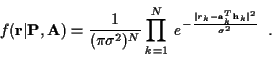 |
(6) |
For a non-time-varying channel, let
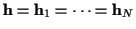 represent the single constant (and unknown) column vector of channel
coefficients, and let
represent the single constant (and unknown) column vector of channel
coefficients, and let
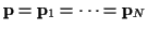 represent the underlying channel coefficient vector.
In this case, using matrix-vector notation,
(1) and (6)
can be expressed more simply as:
represent the underlying channel coefficient vector.
In this case, using matrix-vector notation,
(1) and (6)
can be expressed more simply as:
 |
(7) |
and
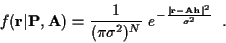 |
(8) |
The basic equations above describe the communication system under
consideration, based only on the facts that the additive noise is white
and Gaussian, and the channel coefficients are linearly-constrained,
but without making any additional assumptions about the
properties of the channel itself.
In the succeeding sections, additional
known properties of the random channel will be considered, starting
from the most general joint pdf case and proceeding to specific examples of
underlying channel coefficient probability distribution functions.
Next: EM and ML Sequence
Up: Sequence Estimation over Linearly-Constrained
Previous: Introduction
Rick Perry
2000-03-16