For each trial in the simulations, random BPSK transmitted symbol values were generated using a uniform distribution, so the symbol values -1 and 1 were equally likely. A channel FIR length of L=3 was used, and the channel was initialized to the known state [-1 -1]. The true noise variance was used for all algorithms.
The Viterbi algorithm, with truncation of the Viterbi trellis at N - L, was used to estimate the transmitted symbols and produce the BER results. For a reference BER, the Viterbi algorithm with known channel coefficients was used.
For comparison purposes, the EM algorithm from [6] was used, and is referred to as ``Kaleh-Vallet'' in the simulation results. The Kaleh-Vallet algorithm produces optimal estimates of the channel coefficients for data blocks which are short enough such that the channel coefficients are non-time-varying over the block. The Viterbi algorithm is then used for MLSE. Also for comparison, the algorithm referred to as ``deterministic'' is that from [1,2,18] and is equivalent to optimal joint sequence and channel estimation . Our EM algorithm for the Gauss-Markov distribution is referred to as ``Gauss-Markov'', and produces optimal estimates of the symbols by marginalizing over the channel coefficient distribution.
The deterministic and Gauss-Markov EM algorithms were initialized using the symbol values as predicted by running the Viterbi algorithm with the true channel coefficients. The Kaleh-Vallet EM algorithm was initialized using the expected value (theoretical average) of the channel coefficients.
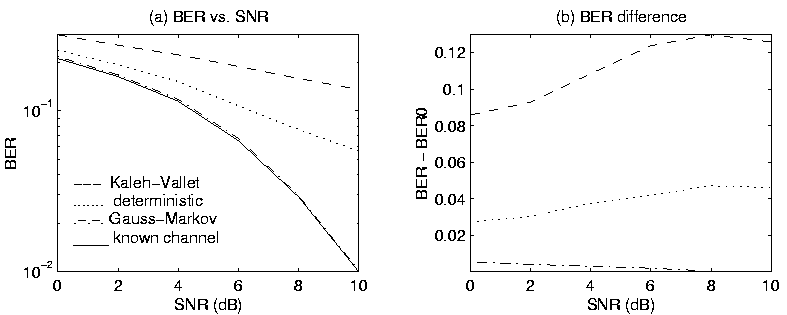 |
For Gauss-Markov channel coefficients, Figure 1
shows results from a typical simulation, and demonstrates that
the Gauss-Markov EM
algorithm performs almost as well as the known channel case,
and much better than the deterministic and Kaleh-Vallet algorithms.
In this simulation, the channel coefficients were generated randomly
using (15) with ![]() having mean
having mean
![]() and covariance
and covariance
![${\bf C} = \left[
\begin{array}{rrr}
0.1 & -0.1 & 0 \\
-0.1 & 0.2 & -0.1 \\
0 & -0.1 & 0.2
\end{array}\right]$](img86.gif) .
.
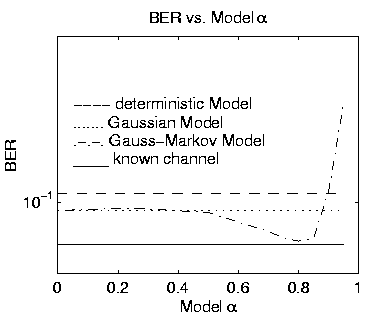
The second simulation illustrates the effect of using an incorrect prior
distribution for the channel coefficients. Using the same parameters
as above to generate the data, with SNR fixed at 6dB, the Gauss-Markov
model used the correct mean and covariance, while ![]() was varied
from 0 to 0.95. Figure 2 shows BER as a function
of model
was varied
from 0 to 0.95. Figure 2 shows BER as a function
of model ![]() .
Also shown are BER
for the time-independent Gaussian [15], deterministic, and known channel estimators
(which are not a function of model
.
Also shown are BER
for the time-independent Gaussian [15], deterministic, and known channel estimators
(which are not a function of model ![]() ).
For model
).
For model ![]() too small or large,
performance is degraded. This should be expected since the marginalization
over
too small or large,
performance is degraded. This should be expected since the marginalization
over ![]() is then based on a prior that does not represent the actual
channel coefficients.
However, for a broad range of
is then based on a prior that does not represent the actual
channel coefficients.
However, for a broad range of ![]() ,
results are better then for
the deterministic model.
For model
,
results are better then for
the deterministic model.
For model
![]() ,
the Gauss-Markov model is
equivalent to the time-independent Gaussian model.
,
the Gauss-Markov model is
equivalent to the time-independent Gaussian model.