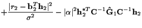
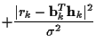
From Section 4 we have
![]() ,
where
,
where
![]() is Gaussian with mean
is Gaussian with mean ![]() and covariance
and covariance ![]() .
Therefore
.
Therefore
![]() is Gaussian with mean
is Gaussian with mean
![]() and covariance
and covariance ![]() .
To derive the formulas for
.
To derive the formulas for ![]() and
and ![]() in this case,
we start by examining the forms of
in this case,
we start by examining the forms of
![]() and
and
![]() .
.
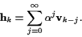
Recursively writing ![]() in terms of
in terms of
![]() ,
,
![]() ,
we obtain:
,
we obtain:
Using Bayes rule,
![]() ,
with:
,
with:
 |
|||
 |
Note that
![]() can be written
in terms of
can be written
in terms of
![]() for any value of k.
(16) shows this for k=1.
In general:
for any value of k.
(16) shows this for k=1.
In general:
To evaluate
![]() ,
we can use the above form of
,
we can use the above form of
![]() in (16) and integrate over
in (16) and integrate over
![]() .
.
Consider two of these integrations, say the integrals over
![]() and
and ![]() .
By examining the form of this result,
we will be able to produce the general
result. Showing just the terms involving
.
By examining the form of this result,
we will be able to produce the general
result. Showing just the terms involving ![]() ,
,
![]() ,
with:
,
with:
| E1 | = | ||
 |
| E1 | |||
Expanding the first term from the exponent in (22),
and dropping constant terms:
| = | |||
| I1 | |||
This result shows how the integral over ![]() produces terms
involving
produces terms
involving ![]() which must be included when performing
the integral over
which must be included when performing
the integral over ![]() .
Showing just the
terms involving
.
Showing just the
terms involving ![]() for this next integral,
for this next integral,
![]() ,
with:
,
with:
| E2 | = | ||
 |
|||
(26) indicates the general form of the equations for
![]() and
and
![]() .
These equations have
more terms than (23) because in deriving (23)
there were no previous integration results to incorporate.
However, if we define
.
These equations have
more terms than (23) because in deriving (23)
there were no previous integration results to incorporate.
However, if we define
![]() and
and
![]() ,
then (23) may also be written in the same form as (26).
,
then (23) may also be written in the same form as (26).
The preceding derivations used (21) to integrate (16)
over ![]() and
and ![]() ,
and show
the recursive forms of the update equations which appear in (19).
If we start at the ``other end'' of (21), and integrate over
,
and show
the recursive forms of the update equations which appear in (19).
If we start at the ``other end'' of (21), and integrate over
![]() first, then
first, then
![]() ,
etc., we
obtain similar recursive equations which appear in (17).
,
etc., we
obtain similar recursive equations which appear in (17).
Finally, to produce
![]() after integrating over
after integrating over
![]() ,
we have
,
we have
![]() ,
with:
,
with:
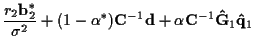
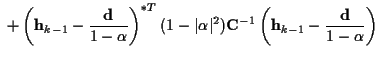
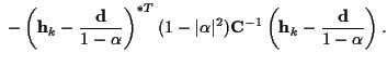
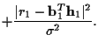
| Ek | = | 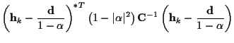 |
|
 |
|||
![$\displaystyle \left[
\frac {{\bf b}_1^* {\bf b}_1^T}
{\sigma^2}
+ {\bf C}^{-1}
\right]^{-1}$](img124.gif)
![$\displaystyle \left[
\frac {{\bf b}_2^* {\bf b}_2^T}
{\sigma^2}
+ {\bf C}^{-1}
...
...t(
{\bf C}^{-1} - {\bf C}^{-1} {\bf\hat{G}}_1 {\bf C}^{-1}
\right)
\right]^{-1}$](img150.gif)