Department of Electrical and Computer Engineering
Villanova University
Villanova, PA 19085

Multitarget List Viterbi Tracking Algorithm

Richard Perry - Anand Vaddiraju - Kevin Buckley

perry(anand, buckley)@ece.vill.edu

Abstract:

In this paper we present an approach to multitarget tracking algorithm development. The approach is based on a trellis diagram which depicts the possible progressions of sequences of location measurements over time. Resulting algorithms are sequential and very flexible in that the approach can handle multiple tracks, track initiation, missed detections, false alarms, and various performance cost functions, while managing computation cost by pruning based on track feasibility. The output of a resulting algorithm can be either a single best set of K tracks, or a list of L best sets of K tracks. The latter is useful, for example, in data fusion where information from other platforms can be used to select one set from the list.

1. Introduction

Multitarget tracking is an important and challenging problem in radar signal processing [1] which is receiving renewed attention within the context of multi-platform system integration (i.e. data fusion). Starting from a time evolving set of noisy detected and false alarm target location/velocity estimates, the problem is to associate the detections over time to form multiple target tracks. For example, maximum likelihood (ML) based data association algorithms have been developed based on track splitting [2], and integer programming [3]. In [1] and [4] algorithms based on a Bayesian formulation have been proposed. In [5], a K-path extension of the Viterbi algorithm is used to find the best K tracks according to a deterministic energy cost function. These approaches identify a set of multiple tracks but do not directly address the possibility that there may be alternative yet reasonable sets of tracks that fit the data nearly as well in the sense optimized to. Such an alternative set of tracks could be the correct set, which in a multiplatform/data-fusion scenario could be determinable with post processing given additional information that would become available.

In this paper we introduce an approach to algorithm development which provides a ranked list of multiple tracks, along with their accompanying costs. The approach is based on a trellis diagram which depicts the possible progressions of sequences of location measurements over time. The processing structure can implement a variety of costs, including ML, Bayesian and deterministic energy. We will focus on maximizing the multitrack likelihood. In this case, trellis branch costs are computed from track innovation processes generated by Kalman filters. Because of the nature of the relationship between measurements and innovations, the Viterbi algorithm can not be used to prune (eliminate from consideration) trellis paths. This is because neither the track innovation nor state processes are Markov. However, a generalization of the Viterbi algorithm termed the list Viterbi algorithm can be used to prune, at each stage and state, all but a subset of tracks called the feasibility tracks.

Below we first describe the tracking problem using an ML formulation. We then describe the trellis diagram based approach, and present a K-track list Viterbi algorithm for ML track estimation. We illustrate this algorithm with a numerical example.

2. Problem Formulation

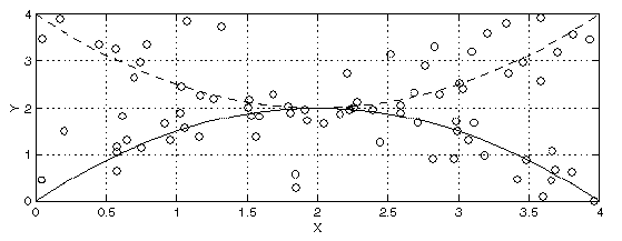
Figure 1 illustrates a tracking scenario with measurements taken over time, plotted as $\cal{X}$ vs. $\cal{Y}$ location coordinates. Two parabolic target tracks are shown. For each target, $\cal{X}$ increases over time. Detections at each time instant consist of noisy measurements of the two targets, along with two false alarms. In general, for detection k at time n, the measurement vector defined as

$${\bf z}_{n,k} = \{z_{n,k,1}, z_{n,k,2},\cdots,z_{n,k,D}\}$$ (1)

may consist of $\cal{X}$ and $\cal{Y}$ coordinates, range and azimuth, velocity parameters etc. The problem we address is to associate detections over time to estimate a set of K target tracks.

  

Figure 1: True tracks and noisy measurements with clutter

Assume that at time index n there are J_n target detections, each of which consists of a set of estimated location/velocity parameters arranged in a measurement vector. We assume that K targets are present. Each detection may be a true target detection or a false alarm. In this paper we assume that for each target and each time n the probability of detection P_D = 1¹.

A candidate track consists of a set of measurements, one taken for each time. At time n, there are $L_n = \prod_{m=1}^{n} J_m$ candidate tracks. Let $\mbox{\boldmath$\theta$ }_n^l ; l=1,2, \cdots, L_n$ represent these, i.e. $\mbox{\boldmath$\theta$ }_n^l = \{ {\bf z}_{1,j_1 (l)} , {\bf z}_{2,j_2 (l)}, \cdots, {\bf z}_{n,j_n (l)} \}$ where j_m (l) indicates the measurement taken from time m for track l, and ${\bf z}_{m,j_m (l)}$ is the j_m (l)measurement vector at time m. So the candidate track l at time n is characterized by $\{ j_1 (l) , j_2 (l) , \cdots, j_n (l) \} .$

Measurement noise is assumed additive, Gaussian and temporally white. For candidate track l the trajectory and measurements are assumed to evolve in time according to the state/measurement equations ²

$${\bf x}_{m+1}^l = {\bf\Phi}_m {\bf x}_m^l + {\bf w}_m^l$$ (2)

$${\bf z}_{m,j_m (l)} = {\bf H}_m {\bf x}_m^l + {\bf v}_m^l$$ (3)

where at time m and for candidate track l, ${\bf x}_m^l$ is the state vector, and ${\bf\Phi}_m$ and ${\bf H}_m$ are the state transition and output matrices respectively. The ${\bf w}_m^l$ and ${\bf v}_m^l$ vectors are zero mean, mutually independent, white and Gaussian with known covariance matrices ${\bf Q}_m$ and ${\bf R}_m$ respectively.

2.1 Single Track Problem

For the single track (K=1) case, given the l^th candidate track is correct, the probability density function of the track measurements $\mbox{\boldmath$\theta$ }_n^l = \{ {\bf z}_{1,j_1 (l)} , {\bf z}_{2,j_2 (l)}, \cdots, {\bf z}_{n,j_n (l)} \}$ is

 

$$p( \mbox{\boldmath$\theta$ }_n^l \vert l ) \prod_{m=1}^n p( {\bf v}_{m,j_m (l)} )$$ = (4)

$$c_n \; exp \left\{ - \frac{1}{2} \sum_{m=1}^{n} {\bf v}_{m,j_m (l)}^T {\bf S}_{m,j_m (l)}^{-1} {\bf v}_{m,j_m (l)} \right\}$$ =

where ${\bf v}_{m,j_m (l)}$ is the innovation of ${\bf z}_{m,j_m (l)}$, ${\bf S}_{m,j_m(l)}$ is its covariance matrix, and c_n is a track independent constant. The ${\bf v}_{m,j_m (l)}$ and ${\bf S}_{m,j_m (l)}^{-1}$ are generated by running a Kalman filter on the l^th candidate track measurement sequence $\mbox{\boldmath$\theta$ }_n^l .$The ML track estimate, $\mbox{\boldmath$\theta$ }_n^{ML}$, is the solution to the problem:

$$\max_{\mbox{\boldmath$\theta$ }_n^l} \; \; \; \; \; \; \; p( \mbox{\boldmath$\theta$ }_n^l \vert l )$$ (5)

which is equivalent to minimizing the -log likelihood:

$$\min_{\mbox{\boldmath$\theta$ }_n^l} \; \; \; \; \; \; \; \Lambda_n^l = \sum_{m=1}^{n} \lambda (j_{m-1} (l) , j_m (l) )$$ (6)

where $\lambda (j_{m-1} (l) , j_m (l) ) = {\bf v}_{m,j_m (l)}^T {\bf S}_{m,j_m (l)}^{-1} {\bf v}_{m,j_m (l)}$ is the incremental cost associated with going, in track $\mbox{\boldmath$\theta$ }_n^l$, from measurement ${\bf z}_{m-1,j_{m-1} (l)}$ at time m-1 to measurement ${\bf z}_{m,j_m (l)}$at time m. To directly solve this ML problem, for each time n, Eq (4) must be evaluated for all L_n candidate tracks.

2.2 K Track Problem

For the K track case, the number of candidate sets of K non-intersecting tracks at time n is I_n, where $I_n = \prod_{m=1}^n\left\{J_m! / (J_m-K)!\right\} / K!$. Let the i^th candidate K-track set be $\mbox{\boldmath$\tau$ }_n^i = \{ \mbox{\boldmath$\theta$ }_n^{l_1 (i)} , \mbox{... ...dmath$\theta$ }_n^{l_2 (i)} , \cdots, \mbox{\boldmath$\theta$ }_n^{l_K (i)} \}.$ Given that track set i is true, the probability density function of the combined $n \times K$ track measurements in $\mbox{\boldmath$\tau$ }_n^i$ is

$$p( \mbox{\boldmath$\tau$ }_n^i \vert i ) = \prod_{p=1}^K \prod_{m=1}^n p( {\bf v}_{m,j_m (l_p (i) )} ) \nonumber$$ (7)

$$= d_n \; exp \left\{ -\frac{1}{2} \sum_{p=1}^K \sum_{m=1}^{n... ...m (l_p (i))}^{-1} {\bf v}_{m,j_m (l_p (i))} \right\} \nonumber$$ (8)

where d_n is a constant independent of track set i.

Generalizing the single track ML problem, the ML K-track estimate, $\mbox{\boldmath$\tau$ }_n^{ML}$, is the solution to the problem:

$$\min_{\mbox{\boldmath$\tau$ }_n^i} \; \; \sum_{p=1}^{K} \Lamb... ...m=1}^{n} \lambda (j_{m-1} (l_p (i) ) , j_m (l_p (i)) ) \; \; .$$ (9)

To directly solve this problem, for each time n, Eq (8) must be evaluated for all I_n candidate K-tracks.

2.3 Trellis Diagram Representation

Consider the trellis diagram in Figure 2 which depicts the possible progressions of sequences of location measurements over time for K=1. Each stage of the trellis corresponds to a measurement time. For K=1, at the m^thstage, each of the J_m measurements corresponds to a state. A branch is a connection from a state at stage m-1 to another state at stage m. At time n, the L_n candidate tracks $\mbox{\boldmath$\theta$ }_n^l ; l=1,2, \cdots, L_n$correspond to the L_n possible paths through the trellis from stage 1 to n. For each track, we assign an incremental cost to each branch. For example, for the l^th candidate track $\mbox{\boldmath$\theta$ }_n^l$, the branch cost from stage m-1 to m (i.e. from state j_m-1 (l) to j_m (l)) is $\lambda (j_{m-1} (l) , j_m (l) )$. It is important to note that since for each candidate track a Kalman filter (which has memory back to the 1^st stage through the Kalman states) is being used to compute the incremental costs, the cost associated with a branch depends on what track is being considered. That is, each branch has multiple costs assigned to it, one for each track through it. The cost of the path $\mbox{\boldmath$\theta$ }_n^l$ is the sum of its branch costs. The ML track estimation problem is now one of finding the minimum-cost path through this trellis.

  

Figure 2: Trellis diagram for K = 1

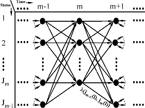For K track estimation, each state of the trellis in Figure 2 is a set of K measurements. So, for stage m with J_m measurements, there are $C(J_m,K)\footnote{$C(A,B)$\space represents the combinations of $A$\space things,taken $B$\space at a time}$ states. Now for each candidate K-track set, the incremental cost assigned to a branch is the sum of the costs of K candidate tracks. So, for candidate K-track set $\mbox{\boldmath$\tau$ }_n^i$, the branch cost from stage m-1 to m is $\sum_{p=1}^{K} \lambda (j_{m-1} (l_p (i) ) , j_m (l_p (i)) )$. As with the K=1 case, the ML K-track estimation problem is now one of finding the minimum-cost path through this trellis.

3. A List Viterbi Tracking Algorithm

Based on the trellis diagram problem formulation described above, we now describe a multitarget ML track estimation algorithm which provides a list of L best K-tracks. The algorithm is sequential, self-initiating and can handle false alarms. Although the algorithm can be modified to compensate for missed detections by employing extra ``absent return'' trellis states, as described here, at each time the algorithm must assign an available measurement (be it an actual detection or false alarm) to each track. In this section a K-track algorithm is described, so that K=1 is treated within this context.

The ML tracking algorithm described in Section 2 would, if solved directly, be computationally prohibitive for large n and even moderate values of K and the J_m 's. Approaches have been proposed to reduce the number of candidate tracks based on feasible tracks [1,2,3]. Effectively, at each time m, the feasible tracks approach eliminates from further consideration the candidate tracks that have too large (i.e. too unlikely) incremental costs at that time. Here we take a similar approach, and implement it within the trellis problem formulation.

The problem is to find the lowest cost path through the trellis. The Viterbi algorithm [7] can be used to sequentially prune the paths through the trellis for certain ML optimization problems (as well as for some other problems). At any stage in the trellis, it keeps only one path to each state. So it is only applicable to problems for which all other paths can not be optimum. It has been used extensively in digital communication and other application problems for which the sequence can be modeled as a Markov process. It has also been proposed for multitarget tracking based on a deterministic energy cost [5], where the incremental path costs from a state j_m-1 at stage m-1 to a state j_m at stage m is a function of only the j_m-1 and j_m measurements.

In general, multitarget tracking problems, couched in a trellis framework, can not be solved using the Viterbi algorithm. For the ML problem considered here, the need for (infinite memory) Kalman filters for each candidate track precludes its use, so that to solve the ML problem at time n an exhaustive search of all L_n paths through the trellis appears necessary. At any stage n in the trellis this requires that we consider all paths into each state at stage n-1, each extended to all states at stage n. That is, the $\prod_{m=1}^{n-1} J_m$ paths into stage n-1 must be extended to the $L_n = \prod_{m=1}^{n} J_m$ paths into stage n, even though the costs of some of these paths will indicate that the corresponding K-track sets are highly unlikely. Alternatively, we propose to keep, at each stage in the trellis, a ``list'' of only the best (lowest cost) L paths to each state, where L is selected to assure that no feasible paths are pruned ³.

Generically, the list Viterbi algorithm [6] does this. The multitarget tracking algorithm we propose incorporates the list Viterbi algorithm, along with the K-track trellis formulation of the multitarget tracking problem [5], and ML cost computation based on Kalman filter innovations [2]. The algorithm determines a list of L feasible K-tracks sets as a list of L paths through the trellis. In general, paths are evaluated according to a defined cost function, where the incremental costs in progressing from stage to stage are computed as branch costs from states to states.

3.1 A Simple Illustrative Example

Here we will apply the algorithm to a simple case consisting of K = 2targets, with measurements spanning 3 instants of time, and find the L = 2best sets of tracks. $({\cal X}_{n,l}, {\cal Y}_{n,l})$ are the $( {\cal X,Y} )$ coordinates of the l^thtarget at time n. Table 1(a) shows these coordinates. We assume the measurement vector ${\bf z}_{n,k}$ consists of $\cal{X}$ and $\cal{Y}$ coordinates only. For the purpose of illustration, we add one clutter/false-alarm measurement at each instant, and assume no measurement noise. Therefore, there are J = 3 measurements per time instant - two actual and one clutter. Table 1(b) shows these measurements.

 

Table 1: (a) Actual positions (b) Measurements (c) Target tracks in terms of measurement indices

 

${\bf\longrightarrow}$ Time	n = 1	n = 2	n = 3
$\downarrow$ Actual Positions
$({\cal{X}}_{n,1},{\cal{Y}}_{n,1})$	(0,0)	(1,1.1)	(2,0)
$({\cal{X}}_{n,2},{\cal{Y}}_{n,2})$	(0,2)	(1,0.9)	(2,2)

(a)

${\bf\longrightarrow}$ Time		n = 1	n = 2	n = 3
$\downarrow$ Measurements
1	(zn,1,1, zn,1,2)	(0,0)	(1.9,1.8)	(0.2,1.6)
2	(zn,2,1, zn,2,2)	(0.4,0.2)	(1,0.9)	(2,0)
3	(zn,3,1, zn,3,2)	(0,2)	(1,1.1)	(2,2)

(b)

Path	State Transition	Measurement Indices
	1,3 $\longrightarrow$ 2,3	1 $\longrightarrow$ 2
Best		3 $\longrightarrow$ 3
	2,3 $\longrightarrow$ 3,2	2 $\longrightarrow$ 3
		3 $\longrightarrow$ 2
	1,3 $\longrightarrow$ 3,2	1 $\longrightarrow$ 3
Second Best		3 $\longrightarrow$ 2
	3,2 $\longrightarrow$ 2,3	3 $\longrightarrow$ 2
		2 $\longrightarrow$ 3

(c)

  

Figure 3: Trellis diagram

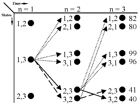Figure 3 shows the trellis structure for this problem. The states at each time instant, representing combinations of the measurement indices (1,2,3) taken two at a time, are denoted by the pairs (1,2), (1,3), and (2,3). The best path(s) to any state must also identify which one of the K! permutations of the measurement indices is being used. This is facilitated in the trellis structure by having two labels, each of which is a different permutation of the combination that the state represents. The states are initialized with 0 path metric at n = 1, therefore only one permutation is shown. For each state at n = 2 and n = 3, we keep the best 2 paths to that state. These paths are marked with dotted-arrows. The numbers at the end of the structure are the path metrics of the best 2 paths to that state.

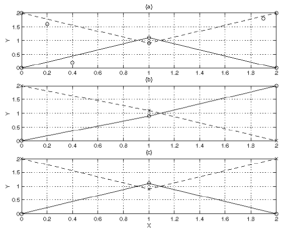
We can now pick the overall best two paths, backtrack through the trellis, and easily identify the sets of target tracks that these state transitions correspond to. Table 1(c) lists these tracks in terms of the measurement indices. Figure 4(a) shows the measurements (actual positions and clutter). Figure 4(b) shows the tracks corresponding to the best path. Notice that at n = 2, there is a switch - the lower and upper estimated tracks follow the upper and lower true tracks, respectively. Figure 4(c) shows the tracks corresponding to the second best path. This path has a slightly higher cost, but resembles the true tracks.

  

Figure 4: (a) True tracks and clutter Measurements (b) Best two tracks, cost=40 (c) 2^nd best two tracks, cost=41

4. An Illustrative Numerical Example

Two parabolic target tracks, consisting of $\cal{X}$ and $\cal{Y}$ position and velocity values, were generated. At each of the 21 time instants, two additional random clutter (false alarm) measurements were generated and random Gaussian noise (variance = 0.01) was added to the target tracks. Figure 1 shows the $\cal{X}$ and $\cal{Y}$ position values for the true tracks and noisy measurements used as input to the algorithm. Velocity values are not shown and, for both tracks, $\cal{X}$ increases with time. Parameter values used were K=2 and L=16.

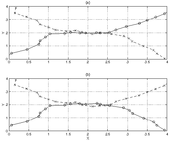
Figure 5(a) shows the best paths. Note that one path starts out following the lower parabolic target then switches to the upper target near the middle of the plot where the target measurements intersect. The total cost of these best paths is 38.5.

Figure 5(b) shows 7^th best paths, which have a cost of 39.3 - just slightly higher than the cost of the best two paths - and correctly follow both the upper and lower parabolic paths. The 2nd through 6th best paths are not shown, since they are very similar to the best path and differ only in a few points.

Our algorithm is able to automatically determine sets of paths with similar costs and dissimilar trajectories by examining the norms of path differences. The differences from the best paths for the 2nd though 16th best paths shows a large jump at index 7 indicating that the 7th best paths significantly differ from the best paths in their trajectory. The cost values for paths 2 through 16 range from 38.7 to 40.3, all just slightly higher than the best paths.

This example demonstrates the usefulness of examining more than just the best set of paths. Sets of paths with similar but slightly higher costs, and dissimilar trajectories, may be passed on to other sensor locations or a data fusion center which could use combined multisensor data to choose the overall most likely set of paths.

  

Figure 5: (a) Best two tracks, cost=38.5 (b) 7^th best two tracks, cost=39.3

5. Conclusions

A novel approach to multitarget tracking, using a trellis structure to find a list of L best sets of K target tracks has been presented. The algorithm described is computationally efficient, and flexibility of the trellis structure facilitates handling track initiation, multiple tracks, false alarms, missed detections and a variety of cost functions. The example presented in Section 4 demonstrates it's usefulness and efficacy in one such model of the problem.