Simulation Results

For all of the simulations shown here, 20,000 trials were performed for values of SNR from 0 to 10 in steps of 2, and two iterations of the EM algorithms were used. For each trial, N = 12 random BPSK transmitted symbol values were generated using a uniform distribution, so the symbol values -1 and 1 were equally likely. A channel FIR length of L=4 was used, the channel was initialized to the known state [-1 -1 -1], and the true noise variance was used in the algorithms. The Viterbi algorithm was used to estimate the transmitted symbols and produce the BER results. For a reference BER, the Viterbi algorithm with known channel coefficients was used. The EM algorithms were initialized using the symbol values as predicted by running the Viterbi algorithm with the true channel coefficients. The channel coefficients were constrained to have a double zero at DC using:

$${\bf F} = \left[ \begin{array}{rrrr} 1 & 1 & 1 & 1 \\ 0 & 1 & 2 & 3 \\ \end{array}\right] , ~ ~ ~ {\bf f} = \left[ \begin{array}{r} 0 \\ 0 \\ \end{array}\right] .$$

  

Figure: 1: BER vs. SNR for deterministic and constrained deterministic EM algorithms using N = 12,   L = 4: (a) absolute BER; (b) BER difference from known channel.

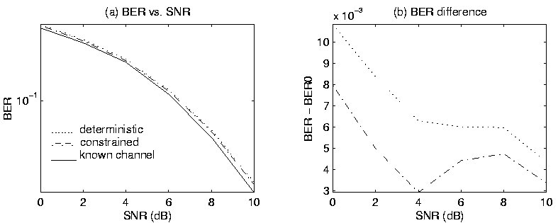For the non-time-varying channel, the first set of simulation results confirm that the EM algorithm which incorporates knowledge of the linear constraints produces lower bit-error-rates in the estimated symbols. For the simulation results shown in Figure 6, ${\bf p}$ was fixed as [1   1]^T. The ``deterministic'' algorithm performs optimal joint sequence and channel estimation [1,12,2] without taking the constraints into account.

  

Figure: 2: BER vs. SNR for deterministic and constrained Gaussian EM algorithms using N = 12,   L = 4: (a) absolute BER; (b) BER difference from known channel.

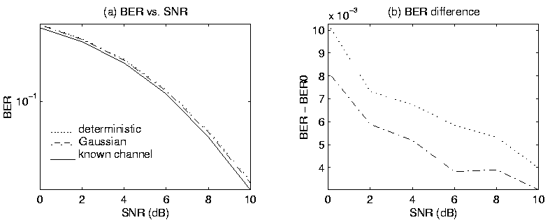In the second set of simulations, the underlying channel coefficients for each trial were generated as Gaussian random values with mean 1 and covariance

$${\bf C} \left[ \begin{array}{rr} 0.5 & -0.5 \\ -0.5 & 1 \\ \end{array}\right] .$$ =

The results shown in Figure 2 demonstrate that when the underlying channel coefficients have a non-time-varying Gaussian distribution, the Gaussian EM algorithm results in lower BER as compared with the EM algorithm for unconstrained deterministic channel coefficients.

  

Figure: 3: BER vs. SNR for deterministic and constrained time-varying Gaussian EM algorithms using N = 12,   L = 4: (a) absolute BER; (b) BER difference from known channel.

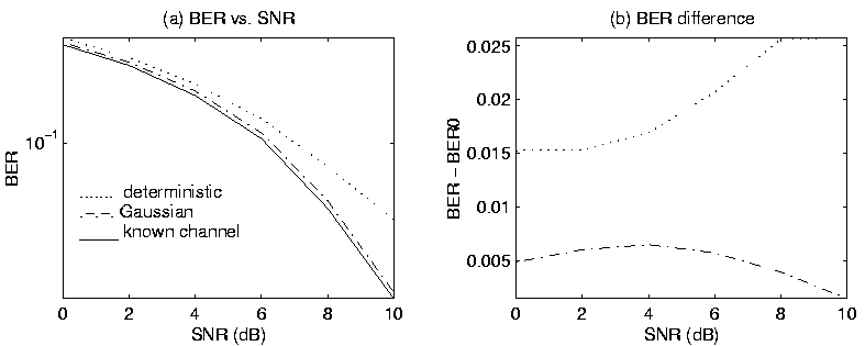For time-varying channel coefficients, Figure 3 shows results from a simulation using the Gaussian EM algorithm. For each trial, the underlying channel coefficients were generated as independent (over time) Gaussian random variables, with mean ${\bf c}_k$ changing linearly from 1 to 2 over the block of time, and fixed covariance

$${\bf C} \left[ \begin{array}{rr} 0.1 & -0.1 \\ -0.1 & 0.2 \end{array}\right] .$$ =

The Gaussian EM algorithm performs almost as well as the known channel in this case, and outperforms the deterministic algorithm dramatically as SNR increases.

  

Figure: 4: BER vs. SNR for deterministic and constrained Gauss-Markov EM algorithms using $N = 12, ~ L = 4, ~ \alpha = 0.8$: (a) absolute BER; (b) BER difference from known channel.

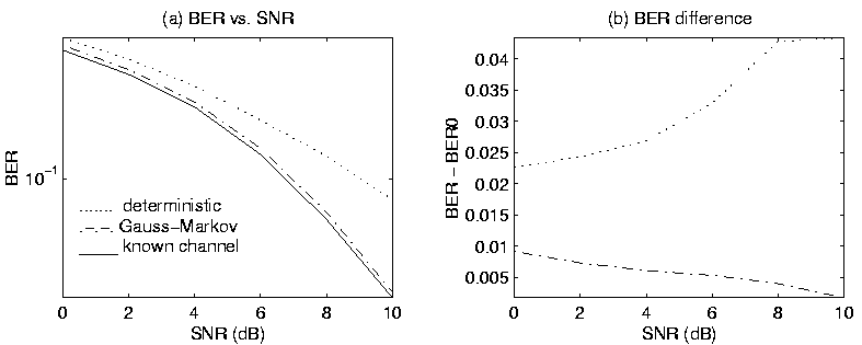For Gauss-Markov channel coefficients, Figure 4 shows results from a typical simulation. The underlying channel coefficients were generated randomly using the Gauss-Markov formula (49) with ${\bf v}_k$ having mean 0.2 and the same covariance matrix as shown above for the time-varying Gaussian simulation. The Gauss-Markov EM algorithm performs almost as well as the known channel case, and much better than the deterministic algorithm.