First Order Gauss Markov Channel Model

Our objective is to incorporate prior knowledge of the fast-fading, FIR channel via a flexible, realistic stochastic linear model that can account for correlation across both channel taps and time. Here we choose a first order Gauss Markov model because it fulfills this objective - it can be used to represent a broad class of fast-varying FIR systems, and the resulting channel taps represent Rayleigh fading.

Let $\alpha$ represent a complex first-order Markov memory factor such that $\vert\alpha\vert = e^{-\omega T}$ where T is the sampling period and $\frac {\omega}{\pi}$ is the Doppler spread [11]. Let the time-varying channel coefficients follow a Gauss-Markov distribution such that, at time k, ${\bf h}_k =\alpha {\bf h}_{k-1} + {\bf v}_k$, where ${\bf v}_k$ is complex, white, and Gaussian with mean $\bf d$ and covariance $E \{ {\bf v}_k {\bf v}_k^H \} = {\bf R}_{\bf v} = \bf C$. In [11] a scalar version of this model is used to represent a frequency-nonselective fast-fading channel. In [12] a slightly different first order Gauss-Markov channel model of a frequency-selective fast-fading channel is used for joint channel/sequence estimation.

For this model, the channel covariance matrix sequence is, in steady state,

$${\bf R}_{\bf h} (m) = E \{ {\bf h}_k {\bf h}_{k+m}^H \} = \f... ...pha^{\vert m\vert}}{1- \vert \alpha \vert^2} {\bf R}_{\bf v} .$$ (5)

For diagonal ${\bf R_{\bf v}}$, the taps weights of the channel are uncorrelated, which for example corresponds to an uncorrelated multipath scattering assumption ([13], p. 842). As indicated above, $\vert \alpha \vert$is selected in accordance with the expected Doppler spread. $\angle \alpha$ controls model Doppler spectrum characteristics.

  

Figure 1: Examples Gauss-Markov channel coefficient trajectories, for channel memory length M=3, for a duration of n=100 symbols, and for $\alpha = 0.95, 0.975, 0.99, 0.995$.

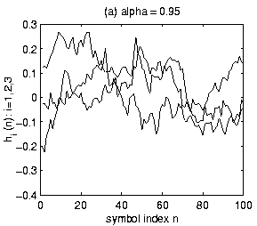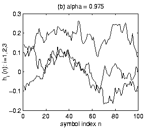
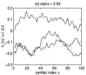
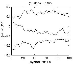
Figure 1 illustrates several M=3 coefficient Gauss-Markov FIR channels. For each, the coefficients are zero-mean (i.e. ${\bf d} = {\bf0}$) and uncorrelated across delay with variances $\sigma_h^2 = 0.01$. Over a n=100symbol duration, example trajectories are plotted for the three coefficients. Figures 1a, 1b, 1c, 1d correspond respectively to $\alpha = 0.95, 0.975, 0.99, 0.995$ and $\omega T = 0.0513, 0.0253, 0.0101, 0.005$. Reliable MAP sequence estimation can not be accomplished for a Gauss-Markov channel with $\alpha = 0.95$. The channel varies too quickly. As expected, as $\alpha$increases towards one, MAP sequence estimation is more reliable. This will be illustrated in the simulation section.