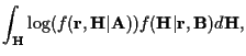
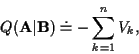
Here we summarize results from [4] and discuss EM convergence for
sequence estimation. To maximize (3) using EM, define the
auxiliary function [9]:
![]() may be written as
may be written as
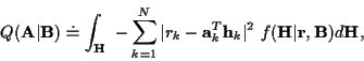
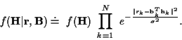
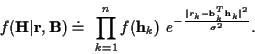
Using (2) in (9) and dropping constants:
A Note on EM Convergence: For discrete or continuous parameter estimation, it was pointed out above that Jensen's inequality holds, proving that at each iteration of the EM algorithm the negative log likelihood function is not increased. For continuous parameter estimation, it is well known the the EM algorithm converges to a minimum or saddle point of the negative log likelihood function (for a proof, see [10]). This proof is based on the global convergence theorem [12], which is now stated.
Let ![]() denote an algorithm on
denote an algorithm on ![]() which, given an initial
estimate
which, given an initial
estimate
![]() generates a sequence
generates a sequence
![]() as
as
![]() .
Let
.
Let
![]() be the solution set. Under the conditions:
be the solution set. Under the conditions:
Let
![]() denote a sequence in the discrete space
denote a sequence in the discrete space
![]() of possible sequence estimates. Let
of possible sequence estimates. Let ![]() represent
the EM algorithm, and
represent
the EM algorithm, and
![]() .
For discrete parameter estimation, condition 1 does not hold since
there is not a compact subset
.
For discrete parameter estimation, condition 1 does not hold since
there is not a compact subset
![]() ,
since
,
since
![]() is a discrete set. As illustrated below, condition 2(a) also
does not hold. This is because
is a discrete set. As illustrated below, condition 2(a) also
does not hold. This is because
![]() is possible when
is possible when
![]() .
Thus, the global convergence theorem is not generally
applicable to the EM algorithm for discrete parameter estimation.
.
Thus, the global convergence theorem is not generally
applicable to the EM algorithm for discrete parameter estimation.
We now show by example
that EM does not necessarily converge to a local discrete minimum
of the negative log likelihood function.
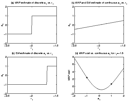
For the independent Gaussian channel model, let
n=1 and M=3, which are small enough to
completely analyze by hand to confirm the results.
A single BPSK symbol a1 at time 1 is to be estimated as either +1 or -1.
The channel is initialized as
![]() -1 -1]T.
For the Gaussian model for the channel coefficients we assume
mean
-1 -1]T.
For the Gaussian model for the channel coefficients we assume
mean
![]() and covariance
and covariance
![]() with v = 0.05.
The noise variance is
with v = 0.05.
The noise variance is
![]() .
The negative log-likelihood cost function of the received data r1
given
.
The negative log-likelihood cost function of the received data r1
given ![]() is obtained from (6)
and (7).
Figure 1(d) illustrates the
MAP cost function for
r1 = -1.8, which is in the range of
r1 where EM breaks down, as discussed below.
is obtained from (6)
and (7).
Figure 1(d) illustrates the
MAP cost function for
r1 = -1.8, which is in the range of
r1 where EM breaks down, as discussed below.
 |
For the EM algorithm, letting ![]() represent an
estimate of
represent an
estimate of ![]() ,
the conditional mean and covariance of
the channel coefficients given the received data are
,
the conditional mean and covariance of
the channel coefficients given the received data are
| = |  |
(17) | |
| = | 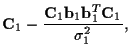 |
(18) |
| (19) |
This example illustrates that for discrete parameter estimation EM
can get stuck at a solution
![]() which is not a local discrete minimum of the negative
log likelihood function. By this we mean that there may be an estimate
which is not a local discrete minimum of the negative
log likelihood function. By this we mean that there may be an estimate
![]() that differs from the EM solution
that differs from the EM solution ![]() in only one element
and that has a lower negative log likelihood cost. We have observed this
phenomenon for EM algorithm solutions to several communications and tracking
related discrete parameter estimation problems. Nonetheless, researchers
have found EM to be useful for discrete
parameter estimation.
The point here is that care must be taken
in employing EM for discrete parameter estimation since convergence to a
minimum of the cost can not be guaranteed.
in only one element
and that has a lower negative log likelihood cost. We have observed this
phenomenon for EM algorithm solutions to several communications and tracking
related discrete parameter estimation problems. Nonetheless, researchers
have found EM to be useful for discrete
parameter estimation.
The point here is that care must be taken
in employing EM for discrete parameter estimation since convergence to a
minimum of the cost can not be guaranteed.