Numerical Examples

Letting J_m = T_mⁱ + F_mⁱ, where T_mⁱ is the number of measurement vectors at time m used in the Ktrack set $\mbox{\boldmath$\tau$ }_n^i$ and F_mⁱ is the number of assumed false alarms, we have that

$$p\left( \mbox{\boldmath$\tau$ }_n^i \right) = \prod_{m=1}^{n} \; P_d^{T_m^i} \; (1-P_d)^{K-T_m^i} \; p( F_m^i ) \; \; ,$$ (16)

where p( F_mⁱ ) is the Poisson distributed probability of F_mⁱfalse alarms. Then, referring to (13), the a priori incremental cost is

 

$$\lambda_m ( \mbox{\boldmath$\tau$ }_n^i ) F_m^i \ln (Y) - T_m^i \ln (P_d )$$ = (17)

$$(K-T_m^i ) \ln (1-P_d ) - \ln (p(F_m^i )) \; \; .$$ -

First, two parabolic target tracks consisting of n=21 ${\cal X}$ and ${\cal Y}$position values were generated. Gaussian measurement noise with a variance of 0.01 was added to the target tracks. ``False detect'' events were generated using a Poisson distribution with a false alarm rate of 2, and the false detections themselves were generated using a uniform distribution over the range [0,4]. Probability of detection was assumed to be 0.7, and for the purpose of illustrating that our algorithm can ``regain'' a target even after a series of missed detections, the lower track was forced to have missed detections from ${\cal X} = 1.5$ to 2.5. Other simulation parameters were K=2 and L=16. Figure 2 shows the ${\cal X}$ and ${\cal Y}$ position values for the true tracks, and the noisy measurements used as input to the algorithm.

  

Figure 2: True Tracks and Measurements

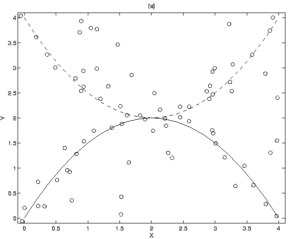Figure 3 shows the best paths, the total cost of which is 117.35. Notice that the one track starts out following the lower target, but switches to the upper target around the region where the true tracks intersect. Figure 4 shows the fourth best paths, which have a total cost of 118.41, just slightly higher than the cost of the best paths, and which correctly follow both the targets. Notice that during missed-detect events, the lower track follows a path tangential to the true track, but ``regains'' the target again when detections are recorded.

  

Figure 3: Best set of two tracks, cost=117.35

  

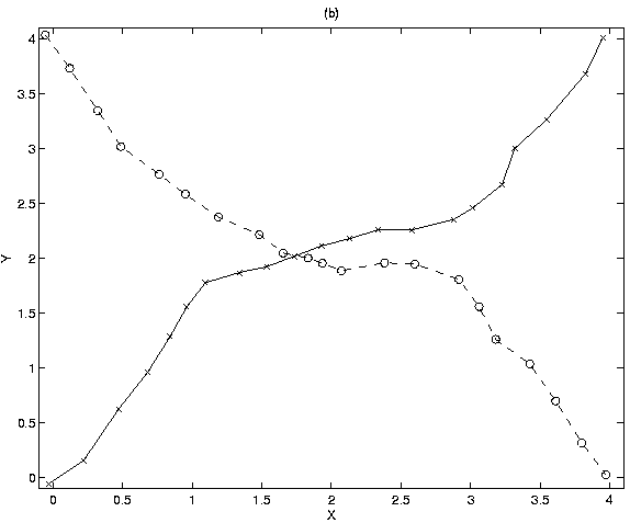Figure 4: 4^th best set of two tracks, cost=118.41.

  

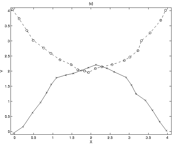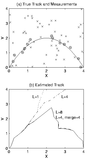
Figure 5: Single Track with Missed Target Events: (a) true track and measurements with false detections; (b) estimated track vs. values of L and merging strategy.

For the second simulation, Figure 5(a) shows an example scenario with a single target traveling in the positive X direction vs. time. In this figure, the solid line is the true target track. ``x'' marks the positions of false detections, which were generated randomly and uniformly over the observation space with a Poisson distribution average of two false detections per unit time. The ``x'''s enclosed in circles represent measurements associated with the target, generated using a noise variance of 0.01. Four sequential missed target events occur in the range $X = 1.4 ~ \ldots ~ 2.0$, and three additional missed target events occur in the range $X = 2.8 ~ \ldots ~ 4.0$. The probability of detection is 0.6.

Figure 5(b) shows the tracks produced by running our algorithm for various values of L and path merging strategy. The track labeled L=1 is from the standard Viterbi algorithm, and the tracks labeled L=4 and L=8 are from our List Viterbi algorithm with no path merging. For L=1 and L=4, the estimated tracks diverge from the true track as soon as the first missed target events occur; they follow the linear predictions from the Kalman filter and/or false detections. For L=8, the estimated track starts to diverge from the true track for $X \ge 1$, then reacquires the true track for $X \ge 2$.

The track labeled L=4, merge=4, is from our List Viterbi algorithm using a track merging period of 4. This track is indistinguishable from the L=8 track, and reacquires the true track with a lower computational and memory cost.