Illustrative Numerical Examples

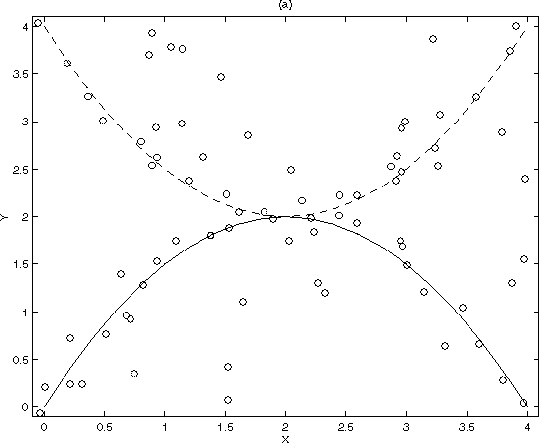
First, two parabolic target tracks consisting of n=21 ${\cal X}$ and ${\cal Y}$ position values were generated. Gaussian measurement noise with a variance of 0.01 was added to the target tracks. ``False detect'' events were generated using a Poisson distribution with a false alarm rate of 2, and the false detections themselves were generated using a uniform distribution over the range [0,4]. Probability of a missed detection was assumed to be 0.3, and for the purpose of illustrating that our algorithm can ``regain" a target even after a series of missed detections, the lower track was forced to have missed detections from ${\cal X} = 1.5$ to 2.5. Other simulation parameters were K=2 and L=16. Figure 2 shows the ${\cal X}$ and ${\cal Y}$ position values for the true tracks, and the noisy measurements used as input to the algorithm.

  

Figure 2: True Tracks and Measurements

Figure 3 shows the best paths, the total cost of which is 117.35. Notice that the one track starts out following the lower target, but switches to the upper target around the region where the true tracks intersect. Figure 4 shows the fourth best paths, which have a total cost of 118.41, just slightly higher than the cost of the best paths, and which correctly follow both the targets. Notice that during missed-detect events, the lower track follows a path tangential to the true track, but ``regains" the target again when detections are recorded.

  

Figure 3: Best set of two tracks, cost=117.35

  

Figure 4: 4^th best set of two tracks, cost=118.41.

Second, Monte Carlo simulations were conducted to compare the Bayesian (21) and marginalization (22) estimates of K. N=25 trials were run per measurement noise value. F K=2 linear tracks were simulated, with n=6 measurement times. Measurement noise variance was 0.01. P_d = 0.7. Poisson distribution with a false alarm rate of 2, and the false detections themselves were generated using a uniform distribution over the range [0,4]. K_max = 4 and L=16. Figure 5 shows estimator performance for varying measurement noise variance. On the basis of these simulations, it can be concluded that estimation by marginalization can be advantageous over Bayesian estimation.

  

Figure 5: Percentage correct estimates of K.

Last, Monte Carlo simulations were run to study K estimator performance for varying probability of detection P_d. N=100 trials were run per P_d value. K=2 linear tracks were simulated, with n=21 measurement times. Measurement noise variance was 0.01. Poisson distribution with a false alarm rate of 1, and the false detections themselves were generated using a uniform distribution over the range [0,4]. K_max = 3 and L=32. Table 1 shows the percentages for different estimates of K vs. P_d.

 

Table 1: Percent correct for the marginalized K estimator:

 

${\bf\longrightarrow}$ K	0	1	2	3
$\downarrow$ Pd
1.00	0	7	93	0
0.95	0	0	96	4
0.90	0	0	91	9
0.85	0	3	85	12
0.80	1	6	72	21