Gaussian Channel Coefficients

Let $f({\bf h})$ be a joint Gaussian distribution with mean $\bf d$ and covariance $\bf C$:

$$f({\bf h}) = \frac {1} {\pi^N \vert{\bf C}\vert} e^{- ({\bf h}-{\bf d})^{*T} {\bf C}^{-1} ({\bf h}-{\bf d}) } ,$$ (29)

where $\bf d$ and $\bf C$ are known. In this case, (12) reduces to:

 

$$f({\bf h}\vert{\bf r},{\bf B}) K_{\ref{eq:f(h\vert r,B)}} ~ e^{- \fr... ...ert{\bf C}\vert} ~ e^{- ({\bf h}-{\bf d})^{*T} {\bf C}^{-1} ({\bf h}-{\bf d}) }$$ =

$$\doteq e^{- ({\bf h}-{\bf g})^{*T} {\bf G}^{-1} ({\bf h}-{\bf g})} ,$$ (30)

with:

  

$${\bf G} \left[ \frac {{\bf B}^{*T} {\bf B}} {{\sigma}^2} + {\bf C}^{-1} \right] ^{-1}$$ = (31)

$${\bf g} {\bf G} \left( \frac {{\bf B}^{*T} {\bf r}} {{\sigma}^2 } + {\bf C}^{-1} {\bf d} \right)$$ = (32)

So in this case, the distribution of ${\bf h}$ given ${\bf r}$ and ${\bf B}$ is also Gaussian. Note that the formula in (32) for the mean of ${\bf h}$ given ${\bf r}$and ${\bf B}$ does not use ${\bf B}^+{\bf r}$ as in the previous deterministic and uniform cases.

The Gaussian distribution of ${\bf h}$ is intermediate between the known deterministic channel case and uniform unknown ${\bf h}$. In the limit as $\bf C$ goes to 0, ${\bf G}$ approaches $\bf C$ and ${\bf g}$ approaches known $\bf d$, which corresponds to the Gaussian distribution approaching $\delta({\bf h}-{\bf d})$. This is similar to the case of deterministic ${\bf h}$ from Section 4.1 except that here the mean is known whereas in Section 4.1 it was estimated using (22). 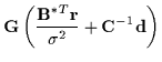In the limit as $\bf C$ goes to infinity, ${\bf G}$ approaches $\left[ \frac {{\bf B}^{*T} {\bf B}}{\sigma^2} \right]^{-1}$and ${\bf g}$ approaches ${\bf B}^+{\bf r}$, which corresponds to the Gaussian distribution approaching a uniform distribution.

Also, if N >> L or the noise variance is small, the term involving ${\bf B}$ in (31) can dominate the ${\bf C}^{-1}$ term, so then ${\bf G}$ approaches $\left[ \frac {{\bf B}^{*T} {\bf B}}{\sigma^2} \right]^{-1}$which approaches 0, and ${\bf g}$ approaches ${\bf B}^+{\bf r}$, which corresponds to the Gaussian EM algorithm becoming equivalent to the algorithm for deterministic channel coefficients.

Therefore, for the case of Gaussian distributed channel coefficients, the EM algorithm is almost the same as for uniform channel coefficients, except that the E-step uses (31) and (32) to estimate ${\bf G}$ and ${\bf g}$.

To use the Viterbi algorithm to initialize ${\bf B}$ in step 1, we could, for example, initialize ${\bf G} = {\bf C}$ and ${\bf g} = {\bf d}$.